plot10 · 代码 1 · 图 0 · 笔记 2 · 代码库专题
单细胞亚群分析
代码库整理的专题,README 见原始目录。
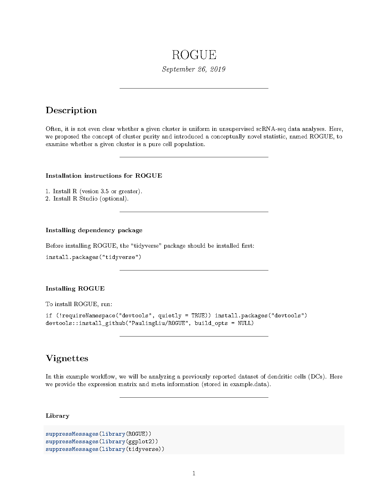
ROGUE Tutorials01_ROGUE/官方源码_ROGUE包/vignettes/ROGUE_Tutorials.pdf
图源:ROGUE_Tutorials.pdf
分析代码
8 个源码文件,按目录顺序;本机绝对路径已替换为 ~。 代码可复制,但需要按自己的数据改路径与参数。
01_rogue/ks教程代码/rogue单细胞纯度分析.r
setwd('D:\\KS项目\\公众号文章\\ROUGE单细胞纯度分析')

#安装包
# if (!requireNamespace("devtools", quietly = TRUE)) install.packages("devtools")
# devtools::install_github("PaulingLiu/ROGUE")

library(Seurat)
library(ROGUE)
library(tidyverse)
library(ggplot2)
library(ggrastr)
#-------------------------------------------------------------------------------
expr <- GetAssayData(Epi, assay = 'RNA',layer = 'counts') %>% as.matrix()
meta <- Epi@meta.data

#filter genes and cells
expr <- matr.filter(expr, min.cells = 10, min.genes = 10)
#-------------------------------------------------------------------------------

ent.res <- SE_fun(expr)
SEplot(ent.res)

#-------------------------------------------------------------------------------
#ROGUE calculation

rogue.value <- CalculateRogue(ent.res, platform = "UMI")


rogue.res <- rogue(expr, labels = meta$seurat_clusters, samples = meta$orig.ident, platform = "UMI", span = 0.6)


#-------------------------------------------------------------------------------
#箱线图可视化结果
#这组颜色来源于cancer cell,可以收藏
myColor <- c("#E41B1B", "#4376AC", "#48A75A", "#87638F", "#D87F32", "#737690", "#D690C6","#B17A7D", "#847A74", "#4285BF","#204B75", "#588257", "#B6DB7B", "#E3BC06", "#FA9B93", "#E9358B", "#A0094E", "#999999", "#6FCDDC", "#BD5E95")


#宽数据转化为长数据格式,使用ggplot作图
plotData <- rogue.res %>%
  tidyr::gather(key = clusters, value = ROGUE) %>%
  filter(!is.na(ROGUE))

#散点箱线图
ggplot(data = plotData, aes(clusters, ROGUE, color = clusters)) +
  geom_boxplot(outlier.shape = NA) +#添加box
  geom_jitter_rast(shape = 16, position = position_jitter(0.2)) +#添加抖动散点
  scale_color_manual(values = myColor) +
  theme_classic() +
  theme(
    axis.text = element_text(size = 12, colour = "black"),
    axis.title = element_text(size = 13, colour = "black")
  ) +
  labs(x = "", y = "ROGUE index") +
  ylim(0, 1)
01_rogue/官方源码_rogue包/r/rogue.r
#' Calculate the expression entropy of each gene
#' @name Entropy
#' @usage Entropy(expr, r = 1)
#' @param expr The expression matrix. Rows should be genes and columns should be cells.
#' @param r A small fixed value to avoid log(0) of mean gene expression levels. The default value of r is set to 1, but can also be set to other values such as 0.1 and 0.01.
#'
#' @return A tibble object with three columns 'Gene', 'mean.expr' and 'entropy'.
#' @export
#'
#' @examples
Entropy <- function(expr, r = 1){
  tmp <- log(expr+1)
  entropy <- Matrix::rowMeans(tmp)
  mean.expr <- log(Matrix::rowMeans(expr)+r)

  ent_res <- tibble(
    Gene = rownames(expr),
    mean.expr = mean.expr,
    entropy = entropy
  )

  return(ent_res)
}


#' Fit the relationship between expression entropy and mean gene expression
#' @name entropy_fit
#' @description Fit the relationship between expression entropy and mean gene expression using loess regression.
#' @usage entropy_fit(.x, span = 0.5, mt.method = c("fdr","BH"))
#' @param .x A tibble object returned from the Entropy function.
#' @param span The parameter α which controls the degree of smoothing.
#' @param mt.method The multiple testing method used in p.adjust.
#' @return A tibble object with six columns.
#' @export
#'
#' @examples ent.res <- Entropy(expr)
#' ent.res <- entropy_fit(ent.res, span = 0.3, mt.method = "fdr")
entropy_fit <- function(.x, span = 0.5, mt.method = "fdr"){
  .x <- .x %>% dplyr::filter(is.finite(mean.expr)) %>% dplyr::filter(entropy > 0)
  fit <- loess(entropy~mean.expr, data = .x, span=span)
  prd <- predict(fit, .x$mean.expr)
  .x %>%
    dplyr::mutate(fit = prd) %>%
    dplyr::mutate(ds = fit - entropy) %>%
    dplyr::mutate(pv = 1-pnorm(.$ds, mean = mean(.$ds), sd = sd(.$ds))) %>%
    dplyr::filter(pv > 0.1) -> tmp

  fit <- loess(entropy~mean.expr, data = tmp, span=span)
  prd <- predict(fit, .x$mean.expr)
  .x %>%
    dplyr::mutate(fit = prd) %>%
    dplyr::mutate(ds = fit - entropy) %>%
    dplyr::filter(is.finite(ds)) %>%
    dplyr::mutate(pv = 1-pnorm(.$ds, mean = mean(.$ds), sd = sd(.$ds))) %>%
    dplyr::filter(pv > 0.1) -> tmp

  fit <- loess(entropy~mean.expr, data = tmp, span=span)
  prd <- predict(fit, .x$mean.expr)

  .x %>%
    dplyr::mutate(fit = prd) %>%
    dplyr::mutate(ds = fit - entropy) %>%
    dplyr::filter(is.finite(ds)) -> .x

  .x <- .x %>% dplyr::mutate(p.value = 1-pnorm(.x$ds, mean = mean(.x$ds), sd = sd(.x$ds)))
  p.adj <- p.adjust(.x$p.value, method = mt.method)
  .x <- .x %>% dplyr::mutate(p.adj = p.adj) %>% dplyr::arrange(desc(ds))
}


#' Identify highly informative genes using S-E model
#' @description Use S-E curve to identify highly informative genes.
#' @param expr The expression matrix. Rows should be genes and columns should be cells.
#' @param span The parameter α which controls the degree of smoothing.
#' @param r A small fixed value to avoid log(0) of mean gene expression levels. The default value of r is set to 1, but can also be set to other values such as 0.1 and 0.01.
#' @param mt.method The multiple testing method used in p.adjust.
#' @param if.adj Whether to apply multiple testing method to adjust p.value.
#' @return A tibble object with seven columns:
#' @return * Gene, the gene name.
#' @return * mean.expr, the mean expression levels of genes.
#' @return * entropy, the expected expression entropy from a given mean gene expression.
#' @return * fit, the mean expression levels of genes.
#' @return * ds, the entropy reduction against the null expectation.
#' @return * p.value, the significance of ds.
#' @return * p.adj, adjusted P value.
#'
#' @export
#'
#' @examples ent.res <- SE_fun(expr, span = 0.1, r = 1, mt.method = "fdr")
SE_fun <- function(expr, span = 0.5, r = 1, mt.method = "fdr", if.adj = T){
  ent_res <- ROGUE::Entropy(expr, r = r)
  ent_res <- ROGUE::entropy_fit(ent_res, span = span, mt.method = mt.method)
  if(!isTRUE(if.adj)){
    ent_res <- ent_res %>% dplyr::mutate(p.adj = p.value)
  }
  return(ent_res)
}


#' S-E plot
#' @description Draws a point plot of the relationship between S and E.
#' @param .x A tibble object returned from the SE_fun or entropy_fit function.
#' @param point_size Point size for geom_point.
#' @param geom_line Logical, whether to show the expected expression entropy.
#' @param p.adj Logical, whether to highlight significantly varied genes.
#' @param cutoff The threshold (adjusted P value) for identifying significantly varied genes.
#'
#' @return A ggplot object
#' @export
#'
#' @examples ent.res <- SE_fun(expr, span = 0.1, r = 1, mt.method = "fdr")
#' SEplot(ent.res)
SEplot <- function(.x, point_size = 1, geom_line = T, p.adj = T, cutoff = 0.05){
  if(isFALSE(p.adj)){
    if(geom_line){
      .x %>%
        ggplot(aes(mean.expr, entropy)) +
        geom_point(colour = '#1E90FF', size = point_size) +
        geom_line(aes(mean.expr, fit), lwd = 0.7) +
        theme_bw() +
        theme(
          axis.title = element_text(size = 15,color="black"),
          axis.text = element_text(size = 15,color="black"),
          legend.title = element_text(size = 0),
          legend.text = element_text(size = 0),
          axis.text.y = element_text(color="black"),
          axis.text.x = element_text(color="black")
        ) +
        labs(
          x = "log(mean expression)",
          y = "expression entropy"
        ) -> p
    }
    else{
      .x %>%
        ggplot(aes(mean.expr, entropy)) +
        geom_point(colour = '#1E90FF', size = point_size) +
        #geom_line(aes(mean.expr, fit), lwd = 0.7) +
        theme_bw() +
        theme(
          axis.title = element_text(size = 15,color="black"),
          axis.text = element_text(size = 15,color="black"),
          legend.title = element_text(size = 0),
          legend.text = element_text(size = 0),
          axis.text.y = element_text(color="black"),
          axis.text.x = element_text(color="black")
        ) +
        labs(
          x = "log(mean expression)",
          y = "expression entropy"
        ) -> p
    }
  }
  if(isTRUE(p.adj)){
    .x <- .x %>% dplyr::mutate(sig = ifelse(p.adj <= cutoff, 1, 0))

    if(geom_line){
      .x %>%
        ggplot(aes(mean.expr, entropy)) +
        geom_point(aes(colour = factor(sig)), size = point_size) +
        geom_line(aes(mean.expr, fit), lwd = 0.7) +
        scale_color_manual(values = c("#1E90FF", "red")) +
        theme_bw() +
        theme(
          legend.position = "none",
          axis.title = element_text(size = 15,color="black"),
          axis.text = element_text(size = 15,color="black"),
          legend.title = element_text(size = 0),
          legend.text = element_text(size = 0),
          axis.text.y = element_text(color="black"),
          axis.text.x = element_text(color="black")
        ) +
        labs(
          x = "log(mean expression)",
          y = "expression entropy"
        ) -> p
    }

    else{
      .x %>%
        ggplot(aes(mean.expr, entropy)) +
        geom_point(aes(colour = factor(sig)), size = point_size) +
        #geom_line(aes(mean.expr, fit), lwd = 0.7) +
        scale_color_manual(values = c("#1E90FF", "red")) +
        theme_bw() +
        theme(
          legend.position = "none",
          axis.title = element_text(size = 15,color="black"),
          axis.text = element_text(size = 15,color="black"),
          legend.title = element_text(size = 0),
          legend.text = element_text(size = 0),
          axis.text.y = element_text(color="black"),
          axis.text.x = element_text(color="black")
        ) +
        labs(
          x = "log(mean expression)",
          y = "expression entropy"
        ) -> p
    }
  }
  return(p)
}


#' Filtering out low-abundance genes and low-quality cells
#'
#' @param expr The expression matrix. Rows should be genes and columns should be cells.
#' @param min.cells Include genes detected in at least this many cells.
#' @param min.genes Include cells where at least this many genes are detected.
#'
#' @return A filtered gene expression matrix.
#' @export
#'
#' @examples expr <- matrix(data = rbinom(n = 100, size = 20, prob = 0.5 ), nrow = 10)
#' expr
#' filtered.expr <- matr.filter(expr, min.cells = 3, min.genes = 3)
#' filtered.expr
matr.filter <- function(expr, min.cells = 10, min.genes = 10){
  gene_count <- colSums(expr > 0, na.rm = T)
  cell_count <- rowSums(expr > 0, na.rm = T)

  lq1 <- cell_count < min.cells
  lq2 <- gene_count < min.genes

  return(expr[!lq1, !lq2])
}


#' ROGUE calculation
#' @description  Using ROGUE to assess the purity of single cell population.
#' @param .x A tibble object returned from the SE_fun or entropy_fit function.
#' @param platform The platform ("UMI" or "full-length") used for generating the tested dataset.
#' @param cutoff The threshold (adjusted P value) for identifying significant ds. The default threshold is 0.05.
#' @param k The scaling factor for calculating ROGUE. The default value of K is set to 45 and 500 for droplet-based ("UMI") and "full-length" based datasets, respectively. When specifying a custom k value, the "platform" argument is redundant.
#' @param features Use these features to calculate ROGUE.
#' @details By taking advantage of the wide applicability of S-E model to scRNA-seq data, we introduce the statistic ROGUE to measure the purity of a cell population as:
#' @details \deqn{ROGUE=1-∑sig.ds/(∑sig.ds+K)}
#' @details where K is an important parameter that constrains the ROGUE value between 0 and 1. A cell population with no significant ds for all genes will receive a ROGUE value of 1, while a population with maximum summarization of significant ds is supposed to yield a purity score of ~0.
#' @return A value of ROGUE.
#' @export
#'
#' @examples ent.res <- SE_fun(expr, span = 0.1, r = 1, mt.method = "fdr")
#' CalculateRogue(ent.res, platform = "UMI")
#' CalculateRogue(ent.res, k = 30)
CalculateRogue <- function(.x, platform = NULL, cutoff = 0.05, k = NULL, features = NULL){
  if(is.null(k)){
    if(is.null(platform)){
      warning("Please provide a \"platform\" argument or specify a k value")
    }else if(platform == "UMI"){
      k = 45
    }else if(platform == "full-length"){
      k = 500
    }else if(!is.null(platform) & !(platform %in% c("UMI","full-length"))){
      warning("Please provide valid \"platform\" argument")
    }
  }else if(!is.null(k)){
    k <- k
  }

  if(!is.null(features)){
    .x <- .x %>% dplyr::filter(Gene %in% features)
    sig_value <- sum(abs(.x$ds))
    Rogue <- 1-sig_value/(sig_value+k)
    return(Rogue)
  }else{
    sig_value <- abs(.x$ds[.x$p.adj < cutoff & .x$p.value < cutoff])
    sig_value <- sum(sig_value)
    Rogue <- 1-sig_value/(sig_value+k)
    return(Rogue)
  }
}


#' Remove outlier cells when calculating ROGUE
#' @usage ent.toli(ent, expr, n = 2, span = 0.5, r = 1, mt.method = c("fdr","BH"))
#' @param ent A tibble object returned from the SE_fun or entropy_fit function.
#' @param expr The expression matrix. Rows should be genes and columns should be cells.
#' @param n Remove this many outlier cells.
#' @param span The parameter α which controls the degree of smoothing.
#' @param r A small fixed value to avoid log(0) of mean gene expression levels. The default value of r is set to 1, but can also be set to other values such as 0.1 and 0.01.
#' @param mt.method The multiple testing method used in p.adjust.
#'
#' @return A tibble object with seven columns as 'ent' object.
#' @export
#'
#' @examples ent.toli(ent.res, expr, n = 2, mt.method = "fdr")
ent.toli <- function(ent, expr, n = 2, span = 0.5, r = 1, mt.method = "fdr"){
  sig.gene <- ent %>% dplyr::filter(p.adj < 0.05) %>% dplyr::pull(Gene)
  ng <- length(sig.gene)
  expr <- expr[sig.gene,]

  mean.v <- c()
  entr.v <- c()
  for (i in 1:ng) {
    .x <- as.numeric(expr[i,])
    .x <- base::sort(.x, decreasing = T)
    .x <- .x[-c(1:n)]
    mean.v[i] <- log(mean(.x)+r)
    entr.v[i] <- mean(log(.x+1))
  }

  mean.cut <- min(ent$mean.expr)

  ent$mean.expr[1:ng] <- mean.v
  ent$entropy[1:ng] <- entr.v

  ent <- ent %>% dplyr::select(-p.adj) %>% dplyr::filter(mean.expr > mean.cut)
  ent <- entropy_fit(ent, span = span, mt.method = "fdr")
  return(ent)
}


#' Calculate the ROGUE value of each putative cluster for each sample.
#' @usage rogue(expr, labels, samples, platform = NULL, k= NULL, min.cell.n = 10, remove.outlier.n = 2, span = 0.5, r = 1, mt.method = c("fdr","BH"))
#' @param expr The expression matrix. Rows should be genes and columns should be cells.
#' @param labels A vector of cell cluster lables for all cells corresponding to 'expr' argument.
#' @param samples A vector of samples (e.g. patients) to which each cell belongs, corresponding to 'expr' argument.
#' @param min.cell.n Only clusters containing at least this many cells will receive ROGUE values.
#' @param remove.outlier.n Remove this many outlier cells when calculating ROGUE.
#' @param span The parameter α which controls the degree of smoothing.
#' @param r A small fixed value to avoid log(0) of mean gene expression levels. The default value of r is set to 1, but can also be set to other values such as 0.1 and 0.01.
#' @param filter Logical, whether to filter out low-abundance genes and low-quality cells.
#' @param min.cells if parameter filter is "TRUE", include genes detected in at least this many cells.
#' @param min.genes if parameter filter is "TRUE", Include cells where at least this many genes are detected.
#' @param mt.method The multiple testing method used in p.adjust.
#'
#' @return A dataframe where rows represent samples, cols represent clusters, and values represent corresponding ROGUEs.
#' @export
#'
#' @examples
rogue <- function(expr, labels, samples, platform = NULL, k = NULL, min.cell.n = 10, remove.outlier.n = 2, span = 0.5, r = 1, filter = F, min.cells = 10, min.genes = 10, mt.method = "fdr"){
  clusters <- unique(labels)
  meta <- tibble(CellID = 1:ncol(expr), ct = labels, sample = samples)
  sample.rogue <- function(meta, cluster){
    tmp <- meta %>% dplyr::filter(ct == cluster)
    s <- unique(samples)
    rogue <- c()
    for (i in 1:length(s)) {
      index1 <- tmp %>% dplyr::filter(sample == s[i]) %>% dplyr::pull(CellID)
      if(length(index1) >= min.cell.n){
        tmp.matr <- expr[,index1]
        if(isTRUE(filter)){
          print("Filtering out low-abundance genes and low-quality cells")
          tmp.matr <- matr.filter(tmp.matr, min.cells = min.cells, min.genes = min.genes)
        }else{
          tmp.matr <- tmp.matr
        }
        tmp.res <- SE_fun(tmp.matr, span = span, r = r)
        tmp.res <- ent.toli(tmp.res, tmp.matr, span = span, r = r, n = remove.outlier.n)
        rogue[i] <- CalculateRogue(tmp.res, platform = platform, k = k)
      }
      else{
        rogue[i] <- NA
      }
    }
    return(rogue)
  }

  res <- list()

  for (i in 1:length(clusters)) {
    res[[i]] <- sample.rogue(meta, clusters[i])
  }

  res.tibble <- Reduce(rbind, res) %>% as.matrix() %>% t() %>% as.data.frame()
  colnames(res.tibble) <- clusters
  rownames(res.tibble) <- unique(samples)
  return(res.tibble)
}


#' Visualize ROGUE values on a boxplot
#' @description Draws a boxplot of the ROGUE values for each cluster in different samples.
#' @param res.rogue A dataframe returned from the 'rogue' function.
#'
#' @return A ggplot object.
#' @export
#'
#' @examples res.rogue <- rogue(expr, labels, samples)
#' rogue.boxplot(res.rogue)
rogue.boxplot <- function(res.rogue){
  res.rogue %>%
    tidyr::gather(key = clusters, value = ROGUE) %>%
    ggplot(aes(clusters, ROGUE)) +
    geom_boxplot(color = "#FF3E96", outlier.shape = NA) +
    geom_point(color = "#FF3E96", size = 1.5) +
    theme_bw() +
    theme(axis.text = element_text(size = 12, colour = "black"),
          axis.title = element_text(size = 13, colour = "black")) +
    labs(
      x = "Clusters",
      y = "ROGUE"
    ) -> p
  return(p)
}


#' Calculate the value of the reference factor K
#' @description Determine the value of the reference factor K by specifying a highly heterogeneous dataset
#' @param expr The expression matrix. Rows should be genes and columns should be cells.
#' @param span The parameter α which controls the degree of smoothing.To improve the performance.
#' @param r A small fixed value to avoid log(0) of mean gene expression levels. The default value of r is set to 1, but can also be set to other values such as 0.1 and 0.01.
#' @param mt.method The multiple testing method used in p.adjust.
#' @param if.adj Whether to apply multiple testing method to adjust p.value.
#' @return The K value
#'
#' @export
#'
#' @examples k <- DetermineK(expr, span = 0.5, r = 1, mt.method = "fdr")
DetermineK <- function(expr, span = 0.5, r = 1, mt.method = "fdr", if.adj = T){
  ent_res <- ROGUE::Entropy(expr, r = r)
  ent_res <- ROGUE::entropy_fit(ent_res, span = span, mt.method = mt.method)
  if(!isTRUE(if.adj)){
    ent_res <- ent_res %>% dplyr::mutate(p.adj = p.value)
  }
  k <- ent_res %>% dplyr::filter(p.adj < 0.05) %>% dplyr::pull(ds) %>% sum()
  k <- k/2
  return(k)
}
01_rogue/官方源码_rogue包/scripts/application.1.fibroblast.analysis.r
library(SingleCellExperiment);library(tidyverse);library(reticulate);library(tidyverse)
library(ggplot2);library(scmap);library(fmsb);library(ggsci);library(ROGUE);library(loomR)
library(Seurat);library(M3Drop);library(ROCR);library(cluster);library(parallel);library(scran)

# Load data
datapath <- "~/projects/04_SEmodel/07_NC_revision/03.data/06.fibroblast"
cell.info <- readr::read_csv(file.path(datapath,"Thienpont_Tumors_52k_v4_R_fixed.cellInfo.txt"))
gene <- readr::read_rds("~/projects/02_data/09_Gene/coding_gene.rds.gz")

dloom <- connect(file.path(datapath,"fibroblasts"), mode = "r")
a <- cell.info %>% dplyr::filter(stringr::str_detect(ClusterName,"fibroblasts"))
a <- as.data.frame(a)
rownames(a) <- a$CellID


sce <- as.Seurat(dloom)
expr <- sce@assays$RNA@counts

overlap.gene <- intersect(gene$gene_name, rownames(expr))
filt.expr <- expr[overlap.gene,]
a <- a[colnames(filt.expr),]

#############
pauling.theme <- function(poi = "right", size = 12, title.size = 13){
  theme(
    legend.position = poi,
    axis.title = element_text(size = title.size,color="black"),
    axis.text = element_text(size = size,color="black"),
    legend.title = element_text(size = size),
    legend.text = element_text(size = size),
    axis.text.y = element_text(color="black"),
    axis.text.x = element_text(color="black"))
}
#############

# OUT path
fig.path <- "~/projects/04_SEmodel/07_NC_revision/02.figures/06.fibroblasts"
out.path <- "~/projects/04_SEmodel/07_NC_revision/03.data/06.fibroblast"

# Clustering (S-E)
filt.expr <- filt.expr[rownames(sce),]
filt.expr <- as.matrix(filt.expr)
ent.res <- SE_fun(filt.expr)

sce.se <- RunPCA(sce, verbose = FALSE, features = ent.res$Gene[1:3000])
sce.se <- RunUMAP(sce.se, dims = 1:30, verbose = FALSE)
pca <- sce.se@reductions$pca@cell.embeddings

adata.com = anndata$AnnData(X=pca, obs=a$PatientNumber)
sc$tl$pca(adata.com)

adata.com$obsm$X_pca = pca
bbknn$bbknn(adata.com,batch_key=0)

sc$tl$umap(adata.com)
sc$tl$leiden(adata.com, resolution = 1.1)
umap.com = py_to_r(adata.com$obsm$X_umap)

tibble::tibble(
  leiden.res.1.bbknn = py_to_r(np$asarray(adata.com$obs$leiden)),
  UMAP1 = umap.com[,1],
  UMAP2 = umap.com[,2]) -> bb.res2

sce.se <- loadumap(sce.se, umap.com, bb.res2)

new.cluster.ids <- paste0("BF_C",c(2,3,1,4,10,9,0,5,6,7,8))
names(new.cluster.ids) <- levels(sce.se)
sce.se <- RenameIdents(sce.se, new.cluster.ids)
DimPlot(sce.se, reduction = "umap", label = TRUE, pt.size = 0.5) + NoLegend()

# save
readr::write_rds(sce, path = file.path(out.path,"01.sce.11.clusters.rds.gz"), compress = "gz")

# Clustering (SCT)
sce <- CreateSeuratObject(counts = filt.expr)
sce <- SCTransform(sce, verbose = FALSE, do.center = F)
sce <- RunPCA(sce, verbose = FALSE)
sce <- RunUMAP(sce, dims = 1:30, verbose = FALSE)
pca <- sce@reductions$pca@cell.embeddings

use_python("~/data/tools/basic/anaconda3/bin/python")
anndata = import("anndata",convert=FALSE)
sc = import("scanpy.api",convert=FALSE)
np = import("numpy",convert=FALSE)
bbknn = import("bbknn", convert=FALSE)
adata.com = anndata$AnnData(X=pca, obs=a$PatientNumber)
sc$tl$pca(adata.com)

adata.com$obsm$X_pca = pca
bbknn$bbknn(adata.com,batch_key=0)

sc$tl$umap(adata.com)
sc$tl$leiden(adata.com, resolution = 1.1)
umap.com = py_to_r(adata.com$obsm$X_umap)

tibble::tibble(
  leiden.res.1.bbknn = py_to_r(np$asarray(adata.com$obs$leiden)),
  UMAP1 = umap.com[,1],
  UMAP2 = umap.com[,2]) -> bb.res

loadumap <- function(.sce, umap, bb.res){
  rownames(umap) <- rownames(.sce@reductions$umap@cell.embeddings)
  colnames(umap) <- colnames(.sce@reductions$umap@cell.embeddings)
  .sce@reductions$umap@cell.embeddings <- umap
  Idents(.sce) <- bb.res$leiden.res.1.bbknn
  return(.sce)
}

sce <- loadumap(sce, umap.com, bb.res)

## Confustion matrix
conf.matr <- table(bb.res$leiden.res.1.bbknn, bb.res2$leiden.res.1.bbknn)
conf.matr <- as.matrix(conf.matr)
conf.matr <- conf.matr/rowSums(conf.matr)
conf.matr %>%
  as.data.frame() %>%
  dplyr::rename(SE = Var1, SCT = Var2) %>%
  ggplot(aes(factor(SCT, levels = c(2,5,10,1,0,3,6,4,7,8,9)), SE)) +
  geom_tile(aes(fill = Freq)) +
  scale_fill_viridis_c() +
  theme_minimal() +
  labs(
    x = "SCT",
    y = "SE"
  ) +
  pauling.theme() -> conf.plot

## UMAP plot
my.cols <- c("#9F79EE", "#00CDCD", "#008B8B", "#FF6EB4", "#B452CD", "#7EC0EE", "#D02090", "#F5DEB3", "#8B864E", "#3CB371","#9BCD9B")
umap.plot1 <- DimPlot(sce.se, label = T, pt.size = 2.3, cols = my.cols) + theme_void() + NoLegend()

ori.sce <- sce.se
Idents(ori.sce) <- a$ClusterID
umap.plot2 <- DimPlot(ori.sce, label = T, pt.size = 2.3, cols = my.cols) + theme_void() + NoLegend()


## Cell type-specific genes
fib.markers <- FindAllMarkers(sce.se, only.pos = TRUE, min.pct = 0.25, logfc.threshold = 0.25, test.use = "t")

top10 <- fib.markers %>% group_by(cluster) %>% top_n(n = 10, wt = avg_logFC)
cell.type.genes.plot <- DoHeatmap(sce.se, features = top10$gene) + NoLegend()

## Marker gene expression
mef2c.plot <- FeaturePlot(sce.se, features = "MEF2C", cols = c("#F0E68C","red"), pt.size = 1.5) + theme_void()
myh11.plot <- FeaturePlot(sce.se, features = "MYH11", cols = c("#F0E68C","red"), pt.size = 1.5) + theme_void()


## ROGUE calculation
rogue.res <- rogue(filt.expr,
                   labels = bb.res2$leiden.res.1.bbknn,
                   samples = a$PatientNumber,
                   platform = "UMI",
                   remove.outlier.n = 5,
                   filter = T,
                   min.cell.n = 20)

av.rogue <- c()
for (i in 1:11) {
  tmp.r <- rogue.res[,i]
  tmp.r <- tmp.r[!is.na(tmp.r)]
  av.rogue[i] <- mean(tmp.r)
}

## ROGUE plot
rogue.plot <- rogue.boxplot(rogue.res) + ylim(0.6,0.97)


## pathway analysis
gs <- readr::read_tsv("/data1/pauling/02_data/18_Enrichment/h.all.v6.2.symbols.gmt", col_names = F)
gs <- gs[,-2]
gs <- gs %>% tidyr::gather(key = "pathway", value = "sets", -X1)
gs <- gs %>% dplyr::filter(sets %in% rownames(sce.se))
table(gs$sets) %>%
  as.data.frame() %>%
  as.tibble() %>%
  dplyr::arrange(desc(Freq)) %>%
  dplyr::filter(Freq == 1) %>%
  dplyr::pull(Var1) -> unique.gene
gs <- gs %>% dplyr::filter(sets %in% unique.gene)

terms <- unique(gs$X1)
geneSets <- list()
for (i in 1:length(terms)) {
  genesets <- gs %>% dplyr::filter(X1 == terms[i]) %>% dplyr::pull(sets)
  geneSets[[terms[i]]] <- genesets
}

y <- as.matrix(sce.se@assays$SCT@data)
gsva_es <- gsva(y, geneSets, mx.diff=1)

sce.gsva <- CreateSeuratObject(counts = gsva_es)
Idents(sce.gsva) <- Idents(sce.se)
fib.markers <- FindAllMarkers(sce.gsva, only.pos = TRUE, min.pct = 0, logfc.threshold = 0.1, test.use = "t")
top10 <- fib.markers %>% group_by(cluster) %>% top_n(n = 10, wt = avg_logFC) %>% dplyr::mutate(gene = stringr::str_replace_all(gene, "-", "_"))
sce.gsva@assays$RNA@scale.data <- gsva_es

tibble(cluster = levels(sce.se)) %>%
  dplyr::mutate(
    expr = purrr::map(
      .x = cluster,
      .f = function(.x){
        tmp.matr <- gsva_es[,Idents(sce.se) == .x]
        rowMeans(tmp.matr)
      }
    )
  ) -> tmp.res

tmp.res <- Reduce(rbind, tmp.res$expr)
tmp.res <- as.data.frame(tmp.res)
rownames(tmp.res) <- levels(sce.se)
tmp.res <- tmp.res[,top10$gene]
tmp.res %>%
  tibble::rownames_to_column(var = "Cluster") %>%
  dplyr::mutate_if(is.numeric, funs((. - mean(.))/sd(.))) %>%
  tidyr::gather(key = "Gene", value = "expr", -Cluster) %>%
  ggplot(aes(factor(Cluster, levels = unique(top10$cluster)), factor(Gene, levels = rev(unique(top10$gene))))) +
  geom_tile(aes(fill = expr), color = "white", lwd = 0.8) +
  #scale_fill_distiller(palette = "Spectral") +
  theme(strip.text.x = element_blank(),
        axis.title = element_text(size = 15),
        axis.text = element_text(size = 9),
        legend.title = element_text(size = 13),
        legend.text = element_text(size = 13),
        axis.text.y = element_text(color = "black"),
        axis.text.x = element_text(color = "black",angle = 45, hjust = 1),
        panel.background = element_rect(colour = "black", fill = "white"),
        panel.grid = element_line(colour = "grey", linetype = "dashed"),
        panel.grid.major = element_line(colour = "grey", linetype = "dashed", size = 0.2)) +
  #facet_grid(. ~ group, scales = "free", space = "free") +
  scale_fill_distiller(palette = "Spectral") +
  labs(x = "", y = "") -> pathway.plot


#############
ggsave(plot = conf.plot, filename = "01.confution.heatmap.pdf", path = fig.path, width = 6, height = 4.5)
ggsave(plot = rogue.plot, filename = "02.se.rogue.box.pdf", path = fig.path, width = 5, height = 4)
ggsave(plot = umap.plot1, filename = "03.re.clustering.se.umap.pdf", path = fig.path, width = 6, height = 4.5)
ggsave(plot = umap.plot2, filename = "04.ori.label.umap.pdf", path = fig.path, width = 6, height = 4.5)
ggsave(plot = mef2c.plot, filename = "05.mef2c.gene.pdf", path = fig.path, width = 5, height = 4)
ggsave(plot = myh11.plot, filename = "05.myh11.gene.pdf", path = fig.path, width = 5, height = 4)
ggsave(plot = cell.type.genes.plot, filename = "06.cell.type.gene.heatmap.pdf", path = fig.path, width = 8, height = 11)
ggsave(plot = pathway.plot, filename = "07.pathway.plot.pdf", path = fig.path, width = 8, height = 8)
01_rogue/官方源码_rogue包/scripts/application.2.bcell.analysis.r
library(SingleCellExperiment);library(tidyverse);library(reticulate);library(tidyverse)
library(ggplot2);library(scmap);library(fmsb);library(ggsci);library(ROGUE)
library(Seurat);library(M3Drop);library(ROCR);library(cluster);library(parallel);library(scran)

# Load data
lung.sce <- readr::read_rds("/data1/pauling/04_SEmodel/01_data/08_lung_Bcells/com.lung.liver.Bcell.rds.gz")
meta <- readr::read_rds("~/projects/04_SEmodel/01_data/08_lung_Bcells/meta.lung.liver.Bcell.rds.gz")
expr <- lung.sce@assays$RNA@counts

# OUT path
fig.path <- "~/projects/04_SEmodel/07_NC_revision/02.figures/07.Bcell"
out.path <- "~/projects/04_SEmodel/07_NC_revision/03.data/07.Bcell"

# Select variable genes using S-E
expr <- as.matrix(expr)
ent.res <- SE_fun(expr)

# Perform clustering with Seurat
lung.se.sce <- RunPCA(lung.sce, verbose = FALSE, features = ent.res$Gene[1:3000])
pca <- lung.se.sce@reductions$pca@cell.embeddings
use_python("~/data/tools/basic/anaconda3/bin/python")
anndata = import("anndata",convert=FALSE)
sc = import("scanpy.api",convert=FALSE)
np = import("numpy",convert=FALSE)
bbknn = import("bbknn", convert=FALSE)
adata.com = anndata$AnnData(X=pca, obs=meta$Donor)
sc$tl$pca(adata.com)

adata.com$obsm$X_pca = pca
bbknn$bbknn(adata.com,batch_key=0)

sc$tl$umap(adata.com, random_state = 3316L)
sc$tl$leiden(adata.com, resolution = 0.8)
umap.com = py_to_r(adata.com$obsm$X_umap)

tibble::tibble(
  leiden.res.1.bbknn = py_to_r(np$asarray(adata.com$obs$leiden)),
  UMAP1 = umap.com[,1],
  UMAP2 = umap.com[,2]) %>%
  dplyr::mutate(Donor = meta$Donor) %>%
  dplyr::mutate(tissue = meta$tissue) %>%
  dplyr::mutate(project = meta$project) -> bb.res

umap.plot <- bb.res %>%
  ggplot(aes(UMAP1, UMAP2)) +
  geom_point(aes(colour = leiden.res.1.bbknn), size = 2) +
  theme_bw() +
  theme_void() +
  theme(legend.position = "none") +
  scale_colour_manual(values = c("#FF83FA", "#66CDAA", "#AB82FF", "#00C5CD", "#00B2EE", "#FF6A6A", "#D02090"))

tis.dist.plot <- bb.res %>%
  ggplot(aes(UMAP1, UMAP2)) +
  geom_point(aes(colour = tissue), size = 2) +
  theme_bw() +
  theme_void() +
  theme(legend.position = "top") +
  scale_colour_manual(values =  c("#00EEEE", "#00B2EE", "#FF69B4", "#FF3E96", "#48D1CC", "#FF8247", "#90EE90"))


# Confusion heatmap
conf.matr <- table(bb.res$leiden.res.1.bbknn, meta$leiden.res.1.bbknn)
conf.matr <- as.matrix(conf.matr)
conf.matr <- conf.matr/rowSums(conf.matr)
conf.matr %>%
  as.data.frame() %>%
  dplyr::rename(SE = Var1, SCT = Var2) %>%
  ggplot(aes(SCT, SE)) +
  geom_tile(aes(fill = Freq)) +
  scale_fill_viridis_c() +
  theme_minimal() -> conf.plot


#ROGUE calculation
bb.res <- bb.res %>% dplyr::mutate(ID = 1:nrow(.))
clusters <- unique(bb.res$leiden.res.1.bbknn)
patient.rogue <- function(info, cluster){
  tmp <- bb.res %>% dplyr::filter(leiden.res.1.bbknn == cluster)
  patients <- unique(bb.res$Donor)
  rogue <- c()
  for (i in 1:length(patients)) {
    print(i)
    index1 <- tmp %>% dplyr::filter(Donor == patients[i]) %>% dplyr::pull(ID)
    if(length(index1) >= 20){
      tmp.matr <- matr[,index1]
      #tmp.matr <- matr.filter(tmp.matr)
      tmp.res <- SE_fun(tmp.matr)
      rogue[i] <- CalculateRogue(tmp.res)
    }
    else{
      rogue[i] <- NA
    }
  }
  return(rogue)
}

res <- list()

for (i in 1:length(clusters)) {
  res[[i]] <- patient.rogue(bb.res, clusters[i])
}

res.tibble <- Reduce(rbind, res) %>% as.matrix() %>% t() %>% as.tibble()
colnames(res.tibble) <- clusters
res.tibble %>%
  tidyr::gather(key = clusters, value = ROGUE) %>%
  ggplot(aes(clusters, ROGUE)) +
  geom_boxplot(color = "#FF3E96", outlier.shape = NA) +
  geom_point(color = "#FF3E96", size = 1.5) +
  theme_bw() +
  theme(axis.text = element_text(size = 12, colour = "black"),
        axis.title = element_text(size = 13, colour = "black")) +
  labs(
    x = "Clusters",
    y = "ROGUE"
  ) -> rogue.plot


# Marker heatmap
Idents(lung.sce) <- bb.res$leiden.res.1.bbknn
b.markers <- FindAllMarkers(lung.sce, only.pos = TRUE, min.pct = 0.25, test.use = "t")
top10 <- b.markers %>%
  dplyr::mutate(cluster = as.character(cluster)) %>%
  group_by(cluster) %>% top_n(n = 10, wt = avg_logFC) %>%
  dplyr::arrange(cluster)

DoHeatmap(lung.sce, top10$gene)
marker.matr <- function(tmp.sce, gene){

  matr <- as.matrix(tmp.sce@assays$SCT@scale.data)
  gene <- intersect(gene, rownames(matr))
  matr <- matr[gene,]

  tibble(cluster = as.numeric(unique(Idents(tmp.sce)))-1) %>%
    dplyr::mutate(
      expr = purrr::map(
        .x = cluster,
        .f = function(.x){
          tmp.matr <- matr[,Idents(tmp.sce) == .x]
          rowMeans(tmp.matr)
        }
      )
    ) -> tmp.res

  matr <- Reduce(rbind, tmp.res$expr)
  matr <- as.data.frame(matr)
  rownames(matr) <- paste("C", tmp.res$cluster, sep = "")
  return(matr)
}
pda <- marker.matr(lung.sce, top10$gene)
pda %>%
  tibble::rownames_to_column(var = "Cluster") %>%
  dplyr::mutate_if(is.numeric, funs((. - mean(.))/sd(.))) %>%
  tidyr::gather(key = "Gene", value = "expr", -Cluster) %>%
  ggplot(aes(Cluster, factor(Gene, levels = rev(unique(top10$gene))))) +
  geom_tile(aes(fill = expr)) +
  #scale_fill_distiller(palette = "Spectral") +
  theme(strip.text.x = element_blank(),
        axis.title = element_text(size = 15),
        axis.text = element_text(size = 9),
        legend.title = element_text(size = 13),
        legend.text = element_text(size = 13),
        axis.text.y = element_text(color = "black"),
        axis.text.x = element_text(color = "black"),
        panel.background = element_rect(colour = "black", fill = "white"),
        panel.grid = element_line(colour = "grey", linetype = "dashed"),
        panel.grid.major = element_line(colour = "grey", linetype = "dashed", size = 0.2)) +
  #facet_grid(. ~ group, scales = "free", space = "free") +
  scale_fill_distiller(palette = "RdBu") +
  labs(x = "", y = "") -> marker.heatmap


# R O/E calculation
meta.sub <- bb.res %>% dplyr::filter(project == "liver")

cluster.table <- table(meta.sub$leiden.res.1.bbknn, meta.sub$tissue)
cluster.table %>%
  as.data.frame() %>%
  dplyr::mutate(
    p.value = purrr::pmap_dbl(
      list(
        .x = Var1,
        .y = Var2,
        .z = Freq
      ),
      .f = function(.x, .y, .z){
        a <- .z
        b <- sum(cluster.table[,.y]) - a
        c <- sum(cluster.table[.x,]) - a
        d <- sum(cluster.table) - a - b - c

        #o <- fisher.test(matrix(c(a, b,c, d), ncol = 2), alternative = "greater")
        #o$estimate
        o <- chisq.test(matrix(c(a, b, c, d), ncol = 2))
        oe <- o$observed/o$expected
        oe[1,1]
      }
    )
  ) -> enrich.res

#adj.p.value <- p.adjust(enrich.res$p.value, method = "BH")
#enrich.res <- enrich.res %>% dplyr::mutate(adj.p.value = adj.p.value)
enrich.res %>%
  dplyr::rename(`Ro/e` = p.value) %>%
  #dplyr::mutate(p.value = ifelse(p.value < 1, -1/p.value, p.value)) %>%
  #dplyr::mutate(`-log10(adj.P-value)` = -log10(adj.p.value)) %>%
  ggplot(aes(Var2, Var1, fill = `Ro/e`)) +
  geom_tile(colour = "white", lwd = 0.8) +
  theme(axis.title = element_text(size = 12)) +
  theme(axis.text = element_text(size = 12)) +
  theme(legend.title = element_text(size = 10)) +
  theme(legend.text = element_text(size = 10)) +
  theme(panel.grid.major = element_blank(),
        panel.grid.minor = element_blank(),
        panel.background = element_blank(),
        axis.ticks = element_blank(),
        axis.title = element_blank()) +
  theme(axis.text.y = element_text(color="black"),
        axis.text.x = element_text(color="black" ,angle = 45, hjust = 1)) +
  scale_fill_distiller(palette = "Spectral") -> roe.plot


# Ro/e barplot
tissues <- unique(bb.res$tissue)
a <- bb.res %>% dplyr::filter(leiden.res.1.bbknn == 2) %>% dplyr::filter(project == "liver")  # [== 2] # [== "Lung"] #
a$tissue <- as.factor(a$tissue)
sda <- table(a$Donor, a$tissue) %>% as.data.frame()
sda %>%
  as.data.frame() %>%
  tidyr::spread(key = "Var2", value = "Freq") %>%
  as.data.frame() %>%
  tibble::column_to_rownames(var = "Var1") -> sda

sda2 <- t(sda) %>% as.data.frame() %>% dplyr::mutate_all(funs((./sum(.))))
rownames(sda2) <- colnames(sda)

tibble(Tissue = tissues[1:5]) %>%
  dplyr::mutate(mean = purrr::map_dbl(.x = Tissue, function(.x){mean(unlist(sda2[.x,]))})) %>%
  dplyr::mutate(sem = purrr::map_dbl(.x = Tissue, function(.x){sd(unlist(sda2[.x,]))/sqrt(5)})) %>%
  dplyr::mutate(ymax = mean+sem) %>%
  dplyr::mutate(ymin = mean-sem) %>%
  ggplot(aes(factor(Tissue, levels = c("Tumor","Lymphnode","Blood", "Normal", "Ascites")), mean)) +
  geom_col(aes(fill = Tissue), colour = "black") +
  scale_fill_manual(values = c("#009ACD", "#EE3A8C", "#EE82EE", "#20B2AA", "#FF7F50")) +
  geom_errorbar(aes(ymin = ymin, ymax = ymax), width = 0.2) +
  theme_minimal() +
  theme(legend.position = "none") +
  theme(axis.title = element_text(size = 12)) +
  theme(axis.text = element_text(size = 12)) +
  theme(legend.title = element_text(size = 10)) +
  theme(axis.text.y = element_text(color="black"),
        axis.text.x = element_text(color="black")) +
  labs(
    x = "",
    y = "Fraction"
  ) +
  ylim(0,0.9) -> liver.c2

rownames(umap.com) <- rownames(lung.sce@reductions$umap@cell.embeddings)
colnames(umap.com) <- colnames(lung.sce@reductions$umap@cell.embeddings)
lung.sce@reductions$umap@cell.embeddings <- umap.com
FeaturePlot(lung.sce, features = c("MKI67","STMN1"), pt.size = 0.8, cols = c("#EEE9BF", "red"))


# Save
bb.res %>% readr::write_rds(file.path(out.path,"01.clustering.res.rds.gz"), compress = "gz")
ggsave(plot = umap.plot, filename = "01.umap.plot.pdf", path = fig.path, width = 6, height = 4.5)
ggsave(plot = tis.dist.plot, filename = "02.tissue.distribution.plot.pdf", path = fig.path, width = 6, height = 5)
ggsave(plot = rogue.plot, filename = "03.rogue.boxplot.pdf", path = fig.path, width = 6, height = 4.5)
ggsave(plot = conf.plot, filename = "04.confution.heatmap.pdf", path = fig.path, width = 6, height = 4.5)
ggsave(plot = marker.heatmap, filename = "05.marker.heatmap.pdf", path = fig.path, width = 8, height = 8)
ggsave(plot = roe.plot, filename = "06.roe.heatmap.pdf", path = fig.path, width = 4, height = 5)
ggsave(plot = liver.c4, filename = "07.liver.c4.pdf", path = fig.path, width = 5, height = 3.7)
ggsave(plot = liver.c2, filename = "08.liver.c2.pdf", path = fig.path, width = 5, height = 3.7)
01_rogue/官方源码_rogue包/scripts/application.3.brain.data.analysis.r
library(ROGUE)
library(Seurat)
library(tidyverse)
library(ggplot2)
library(clusterProfiler)

fig.path <- "~/projects/04_SEmodel/07_NC_revision/02.figures/10.brain"
my.co <- c("#FF8C00", "#D02090", "#FFE7BA", "#00B2EE","#00C5CD",  "#B0E2FF", "#FF83FA","#9FB6CD", "#AB82FF", "#FFC1C1","#00868B","#FF4040", "#3CB371", "#CD9B9B")

load("/data1/et/muris/facs/FACS_all.Robj")
tiss_FACS@meta.data %>%
  tibble::rownames_to_column(var = "barcode") %>%
  dplyr::filter(tissue == "Brain_Non-Myeloid") %>%
  dplyr::rename(label = cell_ontology_class) %>%
  dplyr::select(barcode, tissue, label, mouse.id) -> cda

expr <- tiss_FACS@data
expr <- expr[,cda$barcode]
expr <- exp(expr)-1
expr <- as.matrix(expr)

row.expr <- tiss_FACS@raw.data
row.expr <- row.expr[,cda$barcode]
row.expr <- as.matrix(row.expr)

rogue.brain <- rogue(
  expr,
  labels = cda$label,
  samples = cda$mouse.id,
  min.cell.n = 15,
  platform = "full-length",
  remove.outlier.n = 0
)

brain.clusters <- colnames(rogue.brain)
brain.clusters <- brain.clusters[c(7,5,6,1,3,2,4)]  ## Order

rogue.brain %>%
  tidyr::gather(key = clusters, value = ROGUE) %>%
  ggplot(aes(factor(clusters, levels = brain.clusters), ROGUE)) +
  geom_boxplot(color = "#FF3E96", outlier.shape = NA) +
  geom_point(color = "#FF3E96", size = 1.5) +
  theme_bw() +
  theme(axis.text = element_text(size = 12,colour = "black"),
        axis.title = element_text(size = 13,colour = "black"),
        axis.text.x = element_text(size = 12, colour = "black", angle = 40, hjust = 1)) +
  labs(x = "Clusters", y = "ROGUE") -> p

ggsave(plot = p, filename = "01.overall.rogue.pdf", path = fig.path, width = 3.97, height = 5.1)

cda.oligo <- cda %>% dplyr::filter(label == "oligodendrocyte")
expr.oligo <- expr[,cda$barcode]

#################################### Clustering ################################################

# Feature selection

genes <- rownames(expr.oligo)
genes <- stringr::str_replace_all(genes, "_", "-")
rownames(expr.oligo) <- genes

ent.res <- SE_fun(expr.oligo)    ## Feature selection with S-E

cda <- as.data.frame(cda)
rownames(cda) <- cda$barcode

sce <- CreateSeuratObject(counts = expr.oligo, meta.data = cda)
sce <- NormalizeData(sce, normalization.method = "LogNormalize", scale.factor = 1000000)
sce <- ScaleData(sce, features = genes)
sce <- RunPCA(sce, features = ent.res$Gene[1:1000])
sce <- FindNeighbors(sce, dims = 1:15)
sce <- FindClusters(sce, resolution = 0.5)
sce <- RunUMAP(sce, dims = 1:20)
DimPlot(sce, label = T)


rogue.oligo <- rogue(
  expr.oligo,
  labels = Idents(sce),
  samples = sce$mouse.id,
  min.cell.n = 15,
  platform = "full-length",
  remove.outlier.n = 0
)


rogue.oligo %>%
  tidyr::gather(key = clusters, value = ROGUE) %>%
  dplyr::mutate(clusters = stringr::str_replace_all(clusters,"Cluster","Cluster ")) %>%
  ggplot(aes(clusters, ROGUE)) +
  geom_boxplot(color = "#FF3E96",outlier.shape = NA) +
  geom_point(color = "#FF3E96", size = 1.5) +
  theme_bw() +
  theme(axis.text = element_text(size = 12,colour = "black"),
        axis.title = element_text(size = 13,colour = "black"),
        axis.text.x = element_text(size = 12,colour = "black", angle = 45, hjust = 1)) +
  labs(x = "", y = "ROGUE") -> p

ggsave(plot = p, filename = "05.reclustering.rogue.pdf", path = fig.path, width = 5.67, height = 5.1)

################################

sce %>% readr::write_rds("~/projects/04_SEmodel/07_NC_revision/03.data/09.brain/01.sce.rds.gz", compress = "gz")
new.cluster.ids <- paste0("Cluster", 1:length(levels(sce)))
names(new.cluster.ids) <- levels(sce)
sce <- RenameIdents(sce, new.cluster.ids)
DimPlot(sce, label = F, pt.size = 1) + scale_colour_manual(values = my.co) + theme_void() + NoLegend()

markers <- FindAllMarkers(sce, logfc.threshold = 0.25, min.pct = 0.25,test.use = "t")
top10 <- markers %>% group_by(cluster) %>% top_n(n = 10, wt = avg_logFC)
DoHeatmap(sce, features = top10$gene, size = 4) + NoLegend()
markers %>% readr::write_rds("~/projects/04_SEmodel/07_NC_revision/03.data/09.brain/02.markers.rds.gz", compress = "gz")

markers <- markers %>% dplyr::distinct(gene, .keep_all = T)
entr <- bitr(markers$gene, fromType = "SYMBOL", toType = "ENTREZID", OrgDb='org.Mm.eg.db')
markers <- markers %>% dplyr::inner_join(entr, by = c("gene" = "SYMBOL"))


kegg.fun <- function(.x){
  cluster1 <- markers %>% dplyr::filter(cluster == .x)

  enrich.pathway <- enrichKEGG(
    cluster1$ENTREZID,
    organism = "mmu",
    keyType = "kegg",
    pvalueCutoff = 0.05,
    pAdjustMethod = "BH",
    minGSSize = 10,
    maxGSSize = 500,
    qvalueCutoff = 0.2,
    use_internal_data = FALSE
  )

  enrich.pathway@result %>% dplyr::arrange(p.adjust) -> res
  return(res)
}

res <- kegg.fun("Cluster5")

res %>%
  dplyr::filter(p.adjust < 0.05) %>%
  ggplot(aes(factor(Description, levels = rev(res$Description)), -log10(p.adjust))) +
  geom_col(aes(fill = -log10(p.adjust))) +
  theme_bw() +
  scale_fill_distiller(palette = "Spectral") +
  coord_flip() +
  labs(
    x = " ",
    y = "-log10(p.value)"
  ) +
  theme(
    axis.title = element_text(size = 15,color="black"),
    axis.text = element_text(size = 12,color="black"),
    legend.title = element_text(size = 12),
    legend.text = element_text(size = 12),
    axis.text.y = element_text(color="black"),
    axis.text.x = element_text(color="black")
  )


expr <- sce@assays$RNA@counts
expr <- t(expr)
expr <- 1000000*expr/rowSums(expr)
expr <- as.matrix(expr)
expr <- as.data.frame(expr)
expr <- expr %>% dplyr::mutate(label = Idents(sce))
etest.gene <- scibet::SelectGene(expr, k = 50, r = F)
Marker_heatmap(expr = expr, gene = etest.gene)
01_rogue/官方源码_rogue包/scripts/batch.effect.evaluation.r
library(tidyverse)
library(ROGUE)
library(ggplot2)

# Load data
matr1 <- readr::read_rds("~/projects/04_SEmodel/01_data/04_rogue/10_batch/matr1_con.rds.gz")
matr2 <- readr::read_rds("~/projects/04_SEmodel/01_data/04_rogue/10_batch/matr2_sti.rds.gz")
mda <- rbind(matr1, matr2)

info <- readr::read_tsv("~/projects/04_SEmodel/01_data/04_rogue/10_batch/nbt.4096-S3.txt")
info <- info %>% dplyr::filter(Cell_Name %in% rownames(mda))
info1 <- info %>% dplyr::filter(Stim_Condition == "ctrl")
info2 <- info %>% dplyr::filter(Stim_Condition == "stim")

matr1 <- t(matr1[info1$Cell_Name,])
matr2 <- t(matr2[info2$Cell_Name,])
mda <- t(mda[info$Cell_Name,])


###############################################################################
###                                                                         ###
###                         Batch ~ interferon-beta                         ###
###                                                                         ###
###############################################################################


# ROGUE calculation
rogue.res1 <- rogue(
  matr1,
  labels = info1$Cluster_ID,
  samples = info1$Patient,
  min.cell.n = 20,
  platform = "UMI",
  remove.outlier.n = 0
)

rogue.res2 <- rogue(
  matr2,
  labels = info2$Cluster_ID,
  samples = info2$Patient,
  min.cell.n = 20,
  platform = "UMI",
  remove.outlier.n = 0
)

rogue.res.comb <- rogue(
  mda,
  labels = info$Cluster_ID,
  samples = info$Patient,
  min.cell.n = 20,
  platform = "UMI",
  remove.outlier.n = 0
)

# Group
rogue.res1 <- rogue.res1 %>% dplyr::mutate(Condition = "Batch 1 (ctrl)")
rogue.res2 <- rogue.res2 %>% dplyr::mutate(Condition = "Batch 2 (stim)")
rogue.res.comb <- rogue.res.comb %>% dplyr::mutate(Condition = "Aggregated")

rogue.res <- rogue.res1 %>% dplyr::bind_rows(rogue.res2, rogue.res.comb)


# Boxplot
fig.path <- "~/projects/04_SEmodel/07_NC_revision/02.figures/09.batch/01.pbmc/01.stimulation"
pauling.theme <- function(poi = "right", size = 12, title.size = 13){
  theme(
    legend.position = poi,
    axis.title = element_text(size = title.size,color="black"),
    axis.text = element_text(size = size,color="black"),
    legend.title = element_text(size = size),
    legend.text = element_text(size = size),
    axis.text.y = element_text(color="black"),
    axis.text.x = element_text(color="black"))
}

rogue.res$Condition <- factor(rogue.res$Condition, levels = c("Batch 1 (ctrl)","Batch 2 (stim)","Aggregated"))

#rogue.res %>% readr::write_rds("~/projects/04_SEmodel/07_NC_revision/03.data/08.batch/rogue.rds.gz", compress = "gz")

cell.types <- c("CD14 Mono","CD16 Mono","CD4 Memory T","CD4 Naive T","CD8 T", "DC")
for (i in 1:6) {
  rogue.res %>%
    tidyr::gather(key = "CellTypes", value = "ROGUE", -Condition) %>%
    dplyr::filter(CellTypes == cell.types[i]) %>%
    ggplot(aes(Condition, ROGUE, colour = Condition)) +
    geom_boxplot(aes(fill = Condition), alpha = 0.5) +
    geom_point(aes(colour = Condition)) +
    theme_classic() +
    pauling.theme(poi = "NULL") +
    labs(x = "") +
    scale_colour_manual(values = c("#00688B", "#008B8B", "#CD6839")) +
    scale_fill_manual(values = c("#00688B", "#008B8B", "#CD6839")) +
    labs(
      title = cell.types[i]
    ) +
    theme(plot.title = element_text(hjust = 0.5)) +
    theme(axis.text.x = element_text(color="black", angle = 30, hjust = 1)) -> p

  ggsave(plot = p, filename = paste0(i,".",cell.types[i],".pdf"), path = fig.path, width = 3.3, height = 4.39)
}


# t.test

pv <- list()
for (i in 1:6) {
  t1 <- t.test(rogue.res1[,cell.types[i]], rogue.res.comb[,cell.types[i]], alternative = "greater")
  t2 <- t.test(rogue.res2[,cell.types[i]], rogue.res.comb[,cell.types[i]], alternative = "greater")

  p1 <- t1$p.value
  p2 <- t2$p.value

  pv[[i]] <- c(p1,p2)
}

pv <- Reduce(rbind, pv)
pv <- as.matrix(pv)

colnames(pv) <- c("P.value-1","P.value-2")
rownames(pv) <- use.cell.types


###############################################################################
###                                                                         ###
###                           Batch ~ Patient                               ###
###                                                                         ###
###############################################################################
fig.path2 <- "~/projects/04_SEmodel/07_NC_revision/02.figures/09.batch/01.pbmc/02.individual"

cell.types <- c("CD14 Mono","CD16 Mono","CD4 Memory T","CD4 Naive T","CD8 T", "DC")
patient.number <- length(unique(info1$Patient))

complete.rogue <- list()
for(i in 1:length(cell.types)){
  rep.rogue <- c()
  print(cell.types[i])
  for (n in 1:20) {
    info1 %>%
      dplyr::filter(Cluster_ID == cell.types[i]) %>%
      dplyr::group_by(Patient) %>%
      dplyr::sample_frac(1/patient.number) %>%
      dplyr::pull(Cell_Name) -> cell.names

    tmp.matr <- matr1[,cell.names]
    tmp.ent <- SE_fun(tmp.matr)
    rep.rogue[n] <- CalculateRogue(tmp.ent, platform = "UMI")
    print(rep.rogue[n])
  }
  complete.rogue[[i]] <- tibble(rogue = rep.rogue, cell.type = cell.types[i])
}

complete.rogue <- Reduce(rbind, complete.rogue)
complete.rogue <- complete.rogue %>% dplyr::mutate(Condition = "Aggregated")

rogue.ind <- rogue.res1 %>%
  dplyr::mutate(Condition = "Individual") %>%
  tidyr::gather(key = "cell.type", value = "rogue", -Condition)

rogue.mg <- rbind(rogue.ind, complete.rogue)
rogue.mg$Condition <- factor(rogue.mg$Condition, levels = c("Individual","Aggregated"))

for (i in 1:6) {
  rogue.mg %>%
    dplyr::filter(cell.type == cell.types[i]) %>%
    dplyr::rename(ROGUE = rogue) %>%
    ggplot(aes(Condition, ROGUE, colour = Condition)) +
    geom_boxplot(aes(fill = Condition), alpha = 0.5) +
    geom_point(aes(colour = Condition)) +
    theme_classic() +
    pauling.theme(poi = "NULL") +
    labs(x = "") +
    scale_colour_manual(values = c("#00688B", "#CD6839")) +
    scale_fill_manual(values = c("#00688B", "#CD6839")) +
    labs(
      title = cell.types[i]
    ) +
    theme(plot.title = element_text(hjust = 0.5)) +
    theme(axis.text.x = element_text(color="black", angle = 30, hjust = 1)) -> p

  ggsave(plot = p, filename = paste0(i,".",cell.types[i],".pdf"), path = fig.path2, width = 3.3, height = 4.39)
}
01_rogue/官方源码_rogue包/scripts/clustering.evaluation.rmd
---
title: "R Notebook"
output: html_notebook
---

```{r}
library(SingleCellExperiment);library(tidyverse);library(reticulate);
library(ggplot2);library(scmap);library(fmsb);
library(ggsci);library(scibet);library(Seurat);library(M3Drop);
library(ROCR);library(cluster);library(parallel);library(RaceID);
library(SC3)
```

##CelSeq 2
```{r}
expr <- readr::read_csv("~/projects/04_SEmodel/07_NC_revision/03.data/01.clustering.ari/02.celseq2.3cl/sc_celseq2.count.csv.gz")
gene.name <- expr$Gene
expr <- as.matrix(expr[,-1])
rownames(expr) <- gene.name

cda <- readr::read_csv("~/projects/04_SEmodel/07_NC_revision/03.data/01.clustering.ari/02.celseq2.3cl/sc_celseq2.metadata.csv.gz")
cda <- cda %>% dplyr::select(sample, cell_line) %>% dplyr::rename(label = cell_line)
```

```{r}
t_expr <- t(expr)
res1 <- SE_fun(t_expr, span = 0.2)
res2 <- m3d_fun(t_expr)
res3 <- Gini_fun(t_expr)
res4 <- HVG_fun(t_expr)
res5 <- sct_fun(t_expr)
res6 <- FanoFactor_fun(t_expr)
res7 <- raceid_fun(t_expr)

tibble(method = c("SE","M3Drop","Gini","HVG","SCT","Fano","RaceID"),
       data = list(res1,res2,res3,res4,res5,res6,res7)) -> diff.gene

out.path <- "~/projects/04_SEmodel/07_NC_revision/01.res/02.clustering/02.3cellline.celseq2"
readr::write_rds(diff.gene,file.path(out.path, "01.diff.gene.rds"))
```

###################

RaceID3 Clustering

###################

```{r}
raceid.clustering <- function(expr, var.gene, cda, method = ""){
  n.cluster <- length(unique(cda$label))
  GeneNumber <- c(100,500,1000,1500,2000)
  res <- c()
  for (i in 1:length(GeneNumber)) {
    N <- GeneNumber[i]
    sc <- SCseq(expr[var.gene$Gene[1:N],])
    sc <- filterdata(sc, mintotal = 1, minexpr = 0, minnumber = 0)
    sc <- compdist(sc, FSelect = F, metric="pearson")
    sc <- clustexp(sc, cln=n.cluster, sat=FALSE, bootnr = 20)
    ari <- mclust::adjustedRandIndex(sc@cluster$kpart, cda$label)
    tmp <- tibble(ARI = ari, method = method, Number = N)
    res <- rbind(res,tmp)
  }
  return(res)
}
```

```{r}
race.res1 <- raceid.clustering(expr, diff.gene$data[[1]], cda, diff.gene$method[1])
race.res2 <- raceid.clustering(expr, diff.gene$data[[2]], cda, diff.gene$method[2])
race.res3 <- raceid.clustering(expr, diff.gene$data[[3]], cda, diff.gene$method[3])
race.res4 <- raceid.clustering(expr, diff.gene$data[[4]], cda, diff.gene$method[4])
race.res5 <- raceid.clustering(expr, diff.gene$data[[5]], cda, diff.gene$method[5])
race.res6 <- raceid.clustering(expr, diff.gene$data[[6]], cda, diff.gene$method[6])
race.res7 <- raceid.clustering(expr, diff.gene$data[[7]], cda, diff.gene$method[7])
```

```{r, fig.width=6, fig.height=4}
race.res <- rbind(race.res1,race.res2,race.res3,race.res4,
      race.res5,race.res6,race.res7)

race.res %>% readr::write_rds(file.path(out.path,"02.race.res.rds"))

race.res %>%
  ggplot(aes(Number, ARI)) +
  geom_line(aes(colour = method), lwd = 0.8) +
  geom_point(aes(colour = method), size = 2.5) +
  theme_bw() +
  scale_colour_d3() +
  pauling.theme(angle = 0) -> p
p

fig.path <- "~/projects/04_SEmodel/07_NC_revision/02.figures/02.clustering/01.3cellline.celseq2"
ggsave(plot = p, filename = "02.raceid3.pdf", path = fig.path, width = 6, height = 4)
```

###################

SC3 Clustering

###################

```{r}
sce <- SingleCellExperiment(
    assays = list(
        counts = as.matrix(expr),
        logcounts = log2(as.matrix(expr) + 1)
    )
)
rowData(sce)$feature_symbol <- rownames(sce)
```

```{r}
sc3.clustering <- function(sce, var.gene, cda, method = ""){
  GeneNumber <- c(100,500,1000,1500,2000)
  res <- c()
  for (i in 1:length(GeneNumber)) {
    N <- GeneNumber[i]
    sc <- sce[as.character(var.gene$Gene[1:N]),]
    sc <- sc3(sc, ks = 3, biology = F, gene_filter = F)
    ari <- mclust::adjustedRandIndex(sc$sc3_3_clusters, cda$label)
    tmp <- tibble(ARI = ari, method = method, Number = N)
    res <- rbind(res,tmp)
  }
  return(res)
}

sc3.res1 <- sc3.clustering(sce, diff.gene$data[[1]], cda, diff.gene$method[1])
sc3.res2 <- sc3.clustering(sce, diff.gene$data[[2]], cda, diff.gene$method[2])
sc3.res3 <- sc3.clustering(sce, diff.gene$data[[3]], cda, diff.gene$method[3])
sc3.res4 <- sc3.clustering(sce, diff.gene$data[[4]], cda, diff.gene$method[4])
sc3.res5 <- sc3.clustering(sce, diff.gene$data[[5]], cda, diff.gene$method[5])
sc3.res6 <- sc3.clustering(sce, diff.gene$data[[6]], cda, diff.gene$method[6])
sc3.res7 <- sc3.clustering(sce, diff.gene$data[[7]], cda, diff.gene$method[7])
```

```{r, fig.width=6, fig.height=4}
sc3.res <- rbind(sc3.res1,sc3.res2,sc3.res3,sc3.res4,sc3.res5,sc3.res6,sc3.res7)

sc3.res %>% readr::write_rds(file.path(out.path,"02.sc3.res.rds"))

sc3.res %>%
  ggplot(aes(Number, ARI)) +
  geom_line(aes(colour = method), lwd = 0.8) +
  geom_point(aes(colour = method), size = 2.5) +
  theme_bw() +
  scale_colour_d3() +
  pauling.theme(angle = 0) +
  ylim(0.9,0.98) -> p
p
ggsave(plot = p, filename = "02.sc3.pdf", path = fig.path, width = 6, height = 4)
```

###################

Seurat Clustering

###################

```{r}
Cal.ARI.silh <- function(.x, .y, method = ""){

  ari <- mclust::adjustedRandIndex(Idents(.x), .y$label)
  tibble(ARI = ari, method = method)

}

get.ari.sl <- function(.x, DiffGene, cda, resolution, gene.numbers, method, n.cluster){
  ari.sl.res <- c()
  for (i in 1:length(gene.numbers)) {
    sce.tmp <- RunPCA(.x, features = DiffGene$Gene[1:gene.numbers[i]])
    sce.tmp <- FindNeighbors(sce.tmp, dims = 1:20)
    sce.tmp <- FindClusters(sce.tmp, resolution = resolution)
    if(length(levels(Idents(sce.tmp))) == n.cluster){
      ari.sl <- Cal.ARI.silh(sce.tmp, cda, method) %>%
        dplyr::mutate(Number = gene.numbers[i])

      ari.sl.res <- rbind(ari.sl.res,ari.sl)
    }
  }
  return(ari.sl.res)
}
```

```{r}
sce <- CreateSeuratObject(counts = expr)
sce <- NormalizeData(sce, normalization.method = "LogNormalize", scale.factor = 10000)
all.genes <- rownames(sce)
sce <- ScaleData(sce, features = all.genes, do.center = F, do.scale = F)

sce.se <- RunPCA(sce, features = diff.gene$data[[1]]$Gene[1:30])
sce.se <- FindNeighbors(sce.se, dims = 1:20)
sce.se <- RunUMAP(sce.se, dims = 1:20)
sce.se <- FindClusters(sce.se, resolution = 0.2)
DimPlot(sce.se, reduction = "umap")

GeneNumer <- c(100,500,1000,1500,2000)
se.ari.sl <- get.ari.sl(sce, diff.gene$data[[1]], cda, 0.2, GeneNumer, "SE", 3)
```

```{r}
sce.M3Drop <- RunPCA(sce, features = diff.gene$data[[2]]$Gene[1:30])
sce.M3Drop <- FindNeighbors(sce.M3Drop, dims = 1:20)
sce.M3Drop <- FindClusters(sce.M3Drop, resolution = 0.8)
sce.M3Drop <- RunUMAP(sce.M3Drop, dims = 1:20)
DimPlot(sce.M3Drop)

se.ari.M3D <- get.ari.sl(sce, diff.gene$data[[2]], cda, 0.8, GeneNumer, "M3Drop", 3)
```


```{r}
sce.gini <- RunPCA(sce, features = diff.gene$data[[3]]$Gene[1:30])
sce.gini <- FindNeighbors(sce.gini, dims = 1:20)
sce.gini <- FindClusters(sce.gini, resolution = 0.2)
sce.gini <- RunUMAP(sce.gini, dims = 1:20)
DimPlot(sce.gini, reduction = "umap")

se.ari.gini <- get.ari.sl(sce, diff.gene$data[[3]], cda, 0.2, GeneNumer, "Gini",3)
```

```{r}
sce.hvg <- RunPCA(sce, features = diff.gene$data[[4]]$Gene[1:100])
sce.hvg <- FindNeighbors(sce.hvg, dims = 1:20)
sce.hvg <- RunUMAP(sce.hvg, dims = 1:20)
sce.hvg <- FindClusters(sce.hvg, resolution = 1)
DimPlot(sce.hvg, reduction = "umap")

se.ari.hvg <- get.ari.sl(sce, diff.gene$data[[4]], cda, 1, GeneNumer, "HVG",3)
```

```{r}
sce.sct <- RunPCA(sce, features = diff.gene$data[[5]]$Gene[1:100])
sce.sct <- FindNeighbors(sce.sct, dims = 1:20)
sce.sct <- RunUMAP(sce.sct, dims = 1:20)
sce.sct <- FindClusters(sce.sct, resolution = 0.2)
DimPlot(sce.sct, reduction = "umap")

se.ari.sct <- get.ari.sl(sce, diff.gene$data[[5]], cda, 0.2, GeneNumer, "SCT", 3)
```

```{r}
sce.fano <- RunPCA(sce, features = diff.gene$data[[6]]$Gene[1:100])
sce.fano <- FindNeighbors(sce.fano, dims = 1:20)
sce.fano <- FindClusters(sce.fano, resolution = 0.2)
sce.fano <- RunUMAP(sce.fano, dims = 1:20)
DimPlot(sce.fano, reduction = "umap")

se.ari.fano <- get.ari.sl(sce, diff.gene$data[[6]], cda, 0.2, GeneNumer, "Fano", 3)
```

```{r}
sce.race <- RunPCA(sce, features = diff.gene$data[[7]]$Gene[1:100])
sce.race <- FindNeighbors(sce.race, dims = 1:20)
sce.race <- FindClusters(sce.race, resolution = 0.2)
sce.race <- RunUMAP(sce.race, dims = 1:20)
DimPlot(sce.race, reduction = "umap")

se.ari.race <- get.ari.sl(sce, diff.gene$data[[7]], cda, 0.2, GeneNumer, "RaceID",3)
```


```{r}
pauling.theme <- function(poi = "right", size = 12, title.size = 15, angle){
  theme(
    legend.position = poi,
    axis.title = element_text(size = title.size,color="black"),
    axis.text = element_text(size = size,color="black"),
    legend.title = element_text(size = 12),
    legend.text = element_text(size = 12),
    axis.text.y = element_text(color="black"),
    axis.text.x = element_text(color="black", angle = angle, hjust = 1))
}
```

```{r, fig.width=6, fig.height=4}
seurat.res <- rbind(se.ari.sl, se.ari.gini, se.ari.fano, se.ari.sct,
                    se.ari.race, se.ari.M3D, se.ari.hvg)

seurat.res %>% readr::write_rds(file.path(out.path,"02.seurat.res.rds"))

seurat.res %>%
  ggplot(aes(Number, ARI)) +
  geom_line(aes(colour = method), lwd = 0.8) +
  geom_point(aes(colour = method), size = 2.5) +
  theme_bw() +
  scale_colour_d3() +
  pauling.theme(angle = 0) -> p
p
ggsave(plot = p, filename = "02..seurat.pdf", path = fig.path, width = 6, height = 4)
```
01_rogue/官方源码_rogue包/scripts/cross.validation.r
library(SingleCellExperiment);library(tidyverse);library(reticulate);library(tidyverse)
library(ggplot2);library(scmap);library(fmsb);library(ggsci);library(scibet)
library(Seurat);library(M3Drop);library(ROCR);library(cluster);library(parallel);library(ROGUE)

expr <- readr::read_csv("/data1/pauling/04_SEmodel/07_NC_revision/03.data/01.clustering.ari/GSM3618014_gene_count.csv.gz")
gene.name <- expr$gene_id
expr <- as.matrix(expr[,-1])
rownames(expr) <- gene.name
expr <- t(expr)

cda <- readr::read_csv("/data1/pauling/04_SEmodel/07_NC_revision/03.data/01.clustering.ari/01.10x.5cl/sc_10x_5cl.metadata.csv.gz")
cda <- cda %>%
  dplyr::select(sample, cell_line) %>%
  dplyr::rename(label = cell_line)

expr <- expr[cda$sample,]

m3d_fun <- function(expr){
  expr <- as.matrix(expr)
  expr <- t(expr)
  norm <- M3DropConvertData(expr, is.counts=TRUE)
  DEgenes <- M3Drop::M3DropFeatureSelection(norm, suppress.plot = T, mt_threshold = 2)
  DEgenes <- DEgenes %>%
    dplyr::arrange(p.value)
  return(DEgenes)
}
HVG_fun <- function(expr){
  expr <- t(expr)
  hvg.res <- BrenneckeGetVariableGenes(expr, suppress.plot = T, fdr = 2)
  return(hvg.res)
}
Gini_fun <- function(expr){

  calcul.gini = function(x, unbiased = TRUE, na.rm = FALSE){
    if (!is.numeric(x)){
      warning("'x' is not numeric; returning NA")
      return(NA)
    }
    if (!na.rm && any(na.ind = is.na(x)))
      stop("'x' contain NAs")
    if (na.rm)
      x = x[!na.ind]
    n = length(x)
    mu = mean(x)
    N = if (unbiased) n * (n - 1) else n * n
    ox = x[order(x)]
    dsum = drop(crossprod(2 * 1:n - n - 1,  ox))
    dsum / (mu * N)
  }

  expr <- t(expr)
  ExprM.RawCounts <- expr


  minCellNum = 0
  minGeneNum = 0
  expressed_cutoff = 1
  gini.bi = 0
  log2.expr.cutoffl = 0
  log2.expr.cutoffh = 30
  Gini.pvalue_cutoff = 0.0001
  Norm.Gini.cutoff = 1
  span = 0.9
  outlier_remove = 0.75
  GeneList = 1
  Gamma = 0.9
  diff.cutoff = 1
  lr.p_value_cutoff = 1e-5
  CountsForNormalized = 100000

  ExpressedinCell_per_gene=apply(ExprM.RawCounts,1,function(x) length(x[x > expressed_cutoff ]))
  nonMir = grep("MIR|Mir", rownames(ExprM.RawCounts), invert = T)  # because Mir gene is usually not accurate
  Genelist = intersect(rownames(ExprM.RawCounts)[nonMir],rownames(ExprM.RawCounts)[ExpressedinCell_per_gene >= minCellNum])
  ExpressedGene_per_cell=apply(ExprM.RawCounts[Genelist,],2,function(x) length(x[x>0]))
  ExprM.RawCounts.filter = ExprM.RawCounts[Genelist,ExpressedGene_per_cell >= 0]

  if(gini.bi==0){
    gini = apply(as.data.frame(ExprM.RawCounts.filter), 1, function(x){calcul.gini(as.numeric(x)) } )    #theoretically, gini have very low chance to have a 1 value
    GiniIndex = as.data.frame(cbind(1:dim(ExprM.RawCounts.filter)[1], gini))
  } else {
    GiniIndex1 <- as.data.frame(apply(ExprM.RawCounts.filter, 1, function(x){calcul.gini(as.numeric(x)) } ) )
    GiniIndex2 <- as.data.frame(apply(ExprM.RawCounts.filter+0.00001, 1, function(x){calcul.gini(as.numeric(1/x)) } ) ) #bi directional
    GiniIndex  <- cbind(GiniIndex1, GiniIndex2)
    colnames(GiniIndex)=c("gini1","gini2")
    GiniIndex$gini2_sign = 0 - GiniIndex$gini2;
    GiniIndex$gini = apply(GiniIndex, 1, max)
    GiniIndex <- na.omit(GiniIndex)
    GiniIndex$gini_sign = GiniIndex$gini
    for(genei in 1:dim(GiniIndex)[1])
    {
      GiniIndex[genei, 5] = ifelse(  GiniIndex[genei, 1] > GiniIndex[genei,2], "up-regulation", "down-regulation")
    }
  }

  Maxs          = apply(ExprM.RawCounts.filter,1,max)
  Means         = apply(ExprM.RawCounts.filter,1,mean)
  log2.Maxs     = log2(Maxs+0.1)
  ExprM.Stat1   = as.data.frame(cbind(Maxs,GiniIndex$gini,log2.Maxs))
  colnames(ExprM.Stat1) = c("Maxs","Gini","log2.Maxs")
  ExprM.Stat1 = ExprM.Stat1[ExprM.Stat1$log2.Maxs>log2.expr.cutoffl & ExprM.Stat1$log2.Maxs<=log2.expr.cutoffh ,]  # is this necessary?
  log2.Maxs = ExprM.Stat1$log2.Maxs
  Gini      = ExprM.Stat1$Gini
  Maxs      = ExprM.Stat1$Maxs

  # .3 fitting in max-gini space
  Gini.loess.fit        = loess(Gini~log2.Maxs, span=span, degree=1)
  Normlized.Gini.Score  = Gini.loess.fit$residuals   #residuals = Gini - Gini.fitted
  Gini.fitted           = Gini.loess.fit$fitted
  ExprM.Stat1           = as.data.frame(cbind(ExprM.Stat1[,c("Maxs","Gini", "log2.Maxs")], Normlized.Gini.Score, Gini.fitted))
  colnames(ExprM.Stat1) = c("Maxs","Gini","log2.Maxs", "Norm.Gini", "Gini.fitted")


  ### remove 25% of first round outlier genes, do second round loess
  Gini.loess.fit.residual = residuals(Gini.loess.fit)
  thresh.outlier = quantile(Gini.loess.fit.residual[Gini.loess.fit.residual>0], outlier_remove)
  id.genes.loess.fit = which(Gini.loess.fit.residual < thresh.outlier)
  id.outliers.loess.fit = which(Gini.loess.fit.residual >= thresh.outlier)
  log2.Maxs.genes = log2.Maxs[id.genes.loess.fit]
  log2.Maxs.outliers = log2.Maxs[id.outliers.loess.fit]
  Gini.loess.fit.2 = loess(Gini[id.genes.loess.fit]~log2.Maxs[id.genes.loess.fit], span=span, degree = 1)
  Gini.loess.fit.2.predict = predict(Gini.loess.fit.2)

  Gini.loess.fit.2.x.y = cbind(log2.Maxs.genes,Gini.loess.fit.2.predict)
  Gini.loess.fit.2.x.y.uniq = as.data.frame(unique(Gini.loess.fit.2.x.y))
  Gini.loess.fit.2.x.y.uniq = Gini.loess.fit.2.x.y.uniq[order(Gini.loess.fit.2.x.y.uniq[,1]),]
  log2.Maxs.genes.sorted = log2.Maxs.genes[order(log2.Maxs.genes)]
  Gini.loess.fit.2.predict.sorted = Gini.loess.fit.2.predict[order(log2.Maxs.genes)]
  #using Gini.loess.fit.2 as model, predict gini value for those outlier which are not used for build model.
  #for each max in outliers set, find the id of max value which is most close in fitted data set
  loc.outliers = apply(matrix(log2.Maxs.outliers),1,function(x){
    if(x<max(log2.Maxs.genes.sorted)){
      return(which(log2.Maxs.genes.sorted>=x)[1])
    }else{
      return(which.max(log2.Maxs.genes.sorted))
    }})
  #check the results
  outlier_max_in_fit <- cbind(log2.Maxs.outliers, loc.outliers, log2.Maxs.genes.sorted[loc.outliers])

  #based on Gini.loess.fit.2, predict outliers which was not used for fitting
  Gini.outliers.predict = apply(cbind(seq(length(log2.Maxs.outliers)),log2.Maxs.outliers),1,function(x){
    id = x[1]
    value = x[2]
    if(value == log2.Maxs.genes.sorted[loc.outliers[id]]){
      return(as.numeric(Gini.loess.fit.2.x.y.uniq[which(Gini.loess.fit.2.x.y.uniq$log2.Maxs.genes>=value)[1],2]))
    }else{
      if(loc.outliers[id]>1){
        return(Gini.loess.fit.2.predict.sorted[loc.outliers[id]-1]+(Gini.loess.fit.2.predict.sorted[loc.outliers[id]]-Gini.loess.fit.2.predict.sorted[loc.outliers[id]-1])*(value-log2.Maxs.genes.sorted[loc.outliers[id]-1])/(log2.Maxs.genes.sorted[loc.outliers[id]]-log2.Maxs.genes.sorted[loc.outliers[id]-1]))
      }else{
        return(Gini.loess.fit.2.predict.sorted[2]-(Gini.loess.fit.2.predict.sorted[2]-Gini.loess.fit.2.predict.sorted[1])*(log2.Maxs.genes.sorted[2]-value)/(log2.Maxs.genes.sorted[2]-log2.Maxs.genes.sorted[1]))
      }
    }
  })

  #plot outliers predict results
  outliers.precit.x.y.uniq = as.data.frame(unique(cbind(log2.Maxs.outliers, Gini.outliers.predict)))
  #plot(outliers.precit.x.y.uniq)
  #plot whole fit2
  colnames(outliers.precit.x.y.uniq) = colnames(Gini.loess.fit.2.x.y.uniq)
  Gini.loess.fit.2.full.x.y.uniq = rbind(Gini.loess.fit.2.x.y.uniq, outliers.precit.x.y.uniq)
  #plot(Gini.loess.fit.2.full.x.y.uniq)

  #calcualte Normlized.Gini.Score2
  Normlized.Gini.Score2                        = rep(0,length(Gini.loess.fit.residual))
  Normlized.Gini.Score2[id.genes.loess.fit]    = residuals(Gini.loess.fit.2)
  Normlized.Gini.Score2[id.outliers.loess.fit] = Gini[id.outliers.loess.fit] - Gini.outliers.predict

  Gini.fitted2           = Gini - Normlized.Gini.Score2
  ExprM.Stat1            = as.data.frame(cbind(ExprM.Stat1[,c("Maxs","Gini", "log2.Maxs", "Gini.fitted", "Norm.Gini" )], Gini.fitted2, Normlized.Gini.Score2))
  colnames(ExprM.Stat1)  = c("Maxs","Gini","log2.Maxs", "Gini.fitted","Norm.Gini",  "Gini.fitted2", "Norm.Gini2")
  Gini.pvalue            = pnorm(-abs(scale(ExprM.Stat1$Norm.Gini2, center=TRUE,scale=TRUE)))
  ExprM.Stat2            = cbind(ExprM.Stat1, Gini.pvalue)  #first time use ExprM.Stat2
  colnames(ExprM.Stat2)  = c("Maxs","Gini","log2.Maxs", "Gini.fitted","Norm.Gini",  "Gini.fitted2", "Norm.Gini2", "p.value")

  ExprM.Stat2 %>%
    tibble::rownames_to_column(var = 'Gene') %>%
    dplyr::arrange(p.value)
}
sct_fun <- function(expr){
  expr <- t(expr)
  colnames(expr) <- paste0("Cell",1:ncol(expr))
  sce <- CreateSeuratObject(counts = expr)
  sce <- Seurat::SCTransform(sce, verbose = FALSE, do.center = F, variable.features.n = nrow(sce))
  sce@assays$SCT@meta.features %>%
    tibble::rownames_to_column(var = "Gene") %>%
    dplyr::arrange(desc(residual_variance)) -> sct.res

  return(sct.res)
}
FanoFactor_fun <- function(expr){
  #calculate Fano factor, choose top 1000 Fano genes
  Fano <- apply(expr,2,function(x) var(x)/mean(x))
  Fano <- Fano %>%
    as.data.frame() %>%
    tibble::rownames_to_column(var = "Gene")

  colnames(Fano) <- c("Gene","fano")
  Fano %>% dplyr::filter(!is.na(fano)) %>% dplyr::arrange(desc(fano))
}
raceid_fun <- function(x, mthr = -1){
  uvar  <- function(x,fit){
    err <- coef(summary(fit))[, "Std. Error"]
    2**(coef(fit)[1] + err[1] + log2(x)*(coef(fit)[2] + err[2]) + (coef(fit)[3] + err[3]) * log2(x)**2)
  }

  x <- t(x)
  m <- apply(x, 1, mean)
  v <- apply(x, 1, var)
  ml <- log2(m)
  vl <- log2(v)
  f <- ml > -Inf & vl > -Inf
  ml <- ml[f]
  vl <- vl[f]
  mm <- -8
  repeat {
    fit <- lm(vl ~ ml + I(ml^2))
    if (coef(fit)[3] >= 0 | mm >= mthr) {
      break
    }
    mm <- mm + 0.5
    f <- ml > mm
    ml <- ml[f]
    vl <- vl[f]
  }
  vln <- log2(v) - log2(sapply(m, FUN = uvar, fit = fit))
  tibble(
    Gene = names(vln),
    vln = vln
  ) %>%
    dplyr::filter(!is.na(vln)) %>%
    dplyr::arrange(desc(vln))
}

rf.fun <- function(expr, label, index_id){
  use_python('~/anaconda3/bin/python')
  rf <- import('sklearn.ensemble')
  RF <- rf$RandomForestClassifier

  X_label <- label$label[index_id]
  Y_label <- label$label[-index_id]
  clf <- RF(n_estimators = 200L)

  res1 <- SE_fun(t(expr[index_id,]))
  res2 <- m3d_fun(expr[index_id,])
  res3 <- Gini_fun(expr[index_id,])
  res4 <- HVG_fun(expr[index_id,])
  res5 <- sct_fun(expr[index_id,])
  res6 <- FanoFactor_fun(expr[index_id,])
  res7 <- raceid_fun(expr[index_id,])

  expr <- log2(expr+1)

  tibble(res = list(res1,res2,res3,res4,res5,res6,res7),
         method = c('SE','M3Drop','Gini','HVG','sct','fano','raceid')) %>%
    dplyr::mutate(
      auc = purrr::map(
        .x = res,
        .f = function(.x){
          tmp <- c()
          n <- 0
          for (num in c(30,50,100,200,300,500,1000,5000)) {
            n <- n + 1
            X_train <- as.matrix(expr[index_id, .x$Gene[1:num]])
            X_test <- as.matrix(expr[-index_id, .x$Gene[1:num]])
            clf$fit(X_train, X_label)
            prd <- clf$predict(X_test)
            CohenKappa <- tibble(
              ori = as.character(Y_label),
              prd = prd)

            CohenKappa %>%
              dplyr::filter(ori == prd) %>%
              nrow(.) -> accuracy

            tmp[n] <- accuracy/nrow(CohenKappa)
          }

          tibble(
            num = c(30,50,100,200,300,500,1000,5000),
            acc = tmp
          ) -> tmp

          return(tmp)
        }
      )
    ) %>%
    dplyr::select(-res) -> fin_res

  print("done")
  return(fin_res)
}

acc <- list()
sample.index <- list()

for (i in 1:50) {
  cda %>%
    dplyr::mutate(ID = 1:nrow(.)) %>%
    dplyr::sample_frac(0.7) %>%
    dplyr::pull(ID) -> sample.index[[i]]
}


for (i in 1:50) {
  acc[[i]] <- rf.fun(expr, cda, sample.index[[i]])
  print(i)
}

Reduce(rbind, acc) %>%
  dplyr::mutate(
    auc = purrr::map2(
      .x = method,
      .y = auc,
      .f = function(.x, .y){
        .y %>%
          dplyr::mutate(method = .x)
      }
    )
  ) -> res

res %>% readr::write_rds("~/projects/04_SEmodel/07_NC_revision/01.res/01.featureSelection/01.10x.classification/02.5.cell.line.rds.gz", compress = "gz")