plot13 · 代码 1 · 图 1 · 笔记 1 · 代码库专题
热图与GO富集
代码库整理的专题,README 见原始目录。
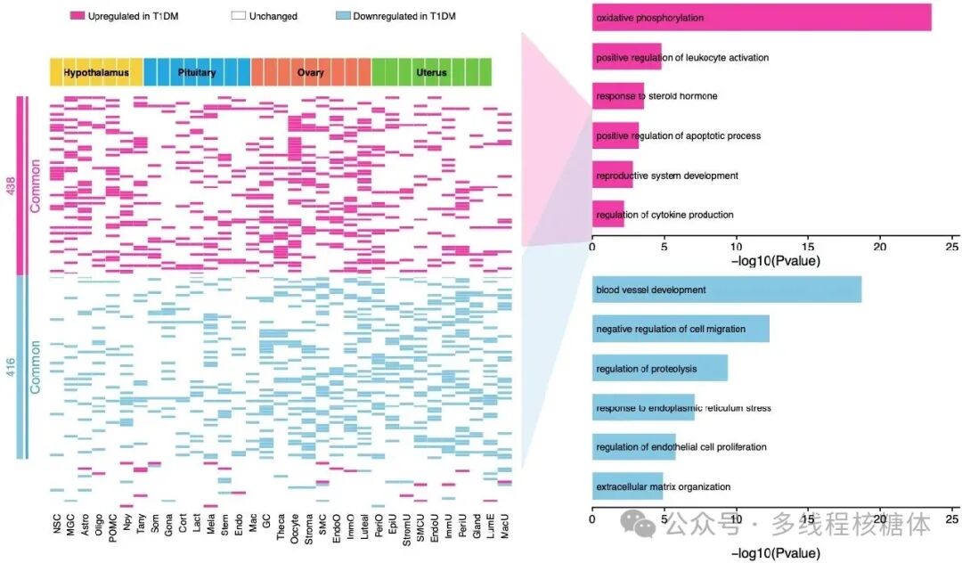
deg heatmap go panel example02_deg_heatmap_go_panel_example.png
图源:02_deg_heatmap_go_panel_example.png
分析代码
1 个源码文件,按目录顺序;本机绝对路径已替换为 ~。 代码可复制,但需要按自己的数据改路径与参数。
01_deg_heatmap_go_panel.r
# ==============================================================================
# 高分 Panel 复现:差异基因热图 + GO 富集放进同一个 Panel
# 对应论文:Single-cell atlas of reproductive endocrine organs reveals
#          transcriptomic responses to type 1 diabetes mellitus in nonhuman
#          primates (Cell Discovery, 2026)
# 来源公众号:Xming同学·多线程核糖体
# 原文链接:https://mp.weixin.qq.com/s/ASViS9MkzqbuQAlh5GudKQ
# ------------------------------------------------------------------------------
# 用途:把【差异基因状态】+【组织来源】+【共同变化基因模块】+【GO 富集】
#       放进同一套视觉结构;GO 条目文字直接叠加在条形区域内部,接近论文排版。
# 输入:3 个 csv(自行准备 / 替换为自己的数据)
#   1. input_cell_annotation.csv : tissue | cell_type | cell_index
#   2. input_deg_heatmap.csv     : gene | module | cell_type | tissue | regulation
#   3. input_go_enrichment.csv   : module | term | neg_log10_p
# 输出:deg_heatmap_go_panel.png / .pdf(7.2 x 4.35 in, 450 dpi)
# 依赖:dplyr, readr, ggplot2, patchwork, grid, scales
# 本地知识库对应笔记:03 生信教程与工具库/02_wiki/tools/可视化与配色/
#                    高分Panel复现-差异基因热图与GO富集组合.md
# ==============================================================================

library(dplyr)
library(readr)
library(ggplot2)
library(patchwork)
library(grid)
library(scales)

# ---- 读取输入 ----------------------------------------------------------------
deg <- read_csv("input_deg_heatmap.csv", show_col_types = FALSE)
cell_anno <- read_csv("input_cell_annotation.csv", show_col_types = FALSE)
go <- read_csv("input_go_enrichment.csv", show_col_types = FALSE)

# ---- 第一步:固定基因和细胞类型顺序 ------------------------------------------
cell_order <- cell_anno$cell_type

gene_order <- deg |>
  distinct(gene, module) |>
  mutate(module = factor(module, levels = c("Common up", "Common down", "Other"))) |>
  arrange(module, gene) |>
  pull(gene)

plot_dat <- deg |>
  mutate(
    cell_type = factor(cell_type, levels = cell_order),
    gene = factor(gene, levels = rev(gene_order)),
    regulation = factor(regulation, levels = c("Upregulated in T1DM", "Unchanged", "Downregulated in T1DM"))
  )

# 模块条坐标(左侧共同基因模块标记)
module_df <- plot_dat |>
  distinct(gene, module) |>
  mutate(y = as.numeric(gene)) |>
  group_by(module) |>
  summarise(ymin = min(y) - 0.5, ymax = max(y) + 0.5, .groups = "drop")

# ---- 第二步:配色 --------------------------------------------------------------
# 热图:粉色=上调,白=未变,蓝=下调
reg_cols <- c(
  "Upregulated in T1DM" = "#f23aa5",
  "Unchanged" = "#ffffff",
  "Downregulated in T1DM" = "#85c8e4"
)
# 组织注释条:独立配色,避免与差异状态混淆
tissue_cols <- c(
  "Hypothalamus" = "#f5cf3d",
  "Pituitary" = "#24a8df",
  "Ovary" = "#f07557",
  "Uterus" = "#70c644"
)

theme_clean <- theme_void(base_size = 8) +
  theme(plot.margin = margin(0, 0, 0, 0))

# ---- 图例行 -------------------------------------------------------------------
legend_dat <- tibble(
  x = c(0.02, 0.42, 0.68),
  label = names(reg_cols),
  fill = unname(reg_cols)
)

p_legend <- ggplot(legend_dat, aes(x = x, y = 0.52)) +
  geom_tile(aes(fill = label), width = 0.034, height = 0.20, color = "grey40", linewidth = 0.13) +
  geom_text(aes(x = x + 0.026, label = label), hjust = 0, size = 1.85, color = "black") +
  scale_fill_manual(values = reg_cols, guide = "none") +
  coord_cartesian(xlim = c(0, 1), ylim = c(0, 1), clip = "off") +
  theme_clean

# ---- 顶部组织注释条 ------------------------------------------------------------
p_tissue <- ggplot(cell_anno, aes(x = factor(cell_type, levels = cell_order), y = 1, fill = tissue)) +
  geom_tile(color = "white", linewidth = 0.22) +
  geom_text(
    data = cell_anno |>
      group_by(tissue) |>
      summarise(x = mean(as.numeric(factor(cell_type, levels = cell_order))), .groups = "drop"),
    aes(x = x, y = 1, label = tissue), inherit.aes = FALSE, size = 1.75, fontface = "bold", color = "black"
  ) +
  scale_fill_manual(values = tissue_cols, guide = "none") +
  scale_x_discrete(expand = c(0, 0)) +
  scale_y_continuous(expand = c(0, 0)) +
  theme_void(base_size = 8) +
  theme(plot.margin = margin(0, 0, 0, 0))

# ---- 中间差异基因热图 -----------------------------------------------------------
p_heat <- ggplot(plot_dat, aes(cell_type, gene, fill = regulation)) +
  geom_tile(color = "#f2f2f2", linewidth = 0.02) +
  # 模块分界白线
  geom_hline(
    yintercept = max(plot_dat |> filter(module == "Common down") |> mutate(y = as.numeric(gene)) |> pull(y)) + 0.5,
    color = "white", linewidth = 0.8
  ) +
  geom_hline(
    yintercept = min(plot_dat |> filter(module == "Common up") |> mutate(y = as.numeric(gene)) |> pull(y)) - 0.5,
    color = "white", linewidth = 0.8
  ) +
  scale_fill_manual(values = reg_cols, guide = "none") +
  scale_x_discrete(expand = c(0, 0)) +
  scale_y_discrete(expand = c(0, 0)) +
  labs(x = NULL, y = NULL) +
  theme_minimal(base_size = 7) +
  theme(
    panel.grid = element_blank(),
    axis.text.y = element_blank(),
    axis.ticks = element_blank(),
    axis.text.x = element_text(angle = 90, vjust = 0.5, hjust = 1, size = 4.8, color = "black"),
    plot.margin = margin(0, 0, 0, 0)
  )

# ---- 左侧模块标记条 -------------------------------------------------------------
p_side <- ggplot(module_df) +
  geom_rect(aes(xmin = 0.28, xmax = 0.42, ymin = ymin, ymax = ymax, fill = module), color = NA) +
  geom_segment(aes(x = 0.50, xend = 0.50, y = ymin, yend = ymax, color = module), linewidth = 0.65) +
  # 基因数量注释(示例 438/416,按实际模块大小替换)
  annotate("text", x = 0.15,
    y = mean(c(min(module_df$ymin[module_df$module == "Common up"]), max(module_df$ymax[module_df$module == "Common up"]))),
    label = "438", color = "#f23aa5", size = 2.15, angle = 90) +
  annotate("text", x = 0.15,
    y = mean(c(min(module_df$ymin[module_df$module == "Common down"]), max(module_df$ymax[module_df$module == "Common down"]))),
    label = "416", color = "#4fa7cc", size = 2.15, angle = 90) +
  annotate("text", x = 0.68,
    y = mean(c(min(module_df$ymin[module_df$module == "Common up"]), max(module_df$ymax[module_df$module == "Common up"]))),
    label = "Common", color = "#f23aa5", size = 2.35, angle = 90) +
  annotate("text", x = 0.68,
    y = mean(c(min(module_df$ymin[module_df$module == "Common down"]), max(module_df$ymax[module_df$module == "Common down"]))),
    label = "Common", color = "#4fa7cc", size = 2.35, angle = 90) +
  scale_fill_manual(values = c("Common up" = "#f23aa5", "Common down" = "#85c8e4", "Other" = "white"), guide = "none") +
  scale_color_manual(values = c("Common up" = "#f23aa5", "Common down" = "#4fa7cc", "Other" = "white"), guide = "none") +
  coord_cartesian(xlim = c(0, 1), ylim = range(module_df$ymin, module_df$ymax), expand = FALSE) +
  theme_void(base_size = 8)

# ---- 右侧 GO 富集条形图 ---------------------------------------------------------
# 核心技巧:GO 文字不放在 y 轴标签,而作为独立文字图层叠加到条形图内部
go_plot <- function(df, fill_col) {
  df <- df |> mutate(term = as.character(term), y = rev(seq_along(term)))

  ggplot(df, aes(y = y)) +
    geom_rect(aes(xmin = 0, xmax = neg_log10_p, ymin = y - 0.34, ymax = y + 0.34),
      fill = fill_col, color = NA) +
    geom_text(aes(x = 0.28, y = y, label = term), hjust = 0, vjust = 0.5, size = 1.62, color = "black") +
    scale_x_continuous(limits = c(0, 25), breaks = seq(0, 25, 5), expand = expansion(mult = c(0, 0.02))) +
    scale_y_continuous(limits = c(0.45, max(df$y) + 0.55), breaks = NULL, expand = c(0, 0)) +
    labs(x = "-log10(Pvalue)", y = NULL) +
    theme_classic(base_size = 8) +
    theme(
      axis.text.y = element_blank(),
      axis.text.x = element_text(size = 6.3, color = "black"),
      axis.title.x = element_text(size = 7.2, color = "black", margin = margin(t = 1)),
      axis.line.y = element_blank(), axis.ticks.y = element_blank(),
      axis.line.x = element_line(linewidth = 0.3), axis.ticks.x = element_line(linewidth = 0.3),
      plot.margin = margin(0, 0, 0, 0)
    )
}

p_go_up <- go_plot(go |> filter(module == "Common up"), "#f23aa5")
p_go_down <- go_plot(go |> filter(module == "Common down"), "#85c8e4")
p_go <- p_go_up / p_go_down

# ---- 连接带(衔接左侧热图与右侧 GO)---------------------------------------------
connector <- function(fill_col, ytop, ybottom) {
  polygonGrob(
    x = unit(c(0, 1, 1, 0), "npc"),
    y = unit(c(ytop, 0.78, 0.52, ybottom), "npc"),
    gp = gpar(fill = alpha(fill_col, 0.24), col = NA)
  )
}

p_link <- ggplot() +
  annotation_custom(connector("#f23aa5", 0.93, 0.51), xmin = 0, xmax = 1, ymin = 0, ymax = 1) +
  annotation_custom(connector("#85c8e4", 0.49, 0.07), xmin = 0, xmax = 1, ymin = 0, ymax = 1) +
  coord_cartesian(xlim = c(0, 1), ylim = c(0, 1), expand = FALSE) +
  theme_void()

# ---- 组合 ----------------------------------------------------------------------
legend_row <- plot_spacer() + p_legend + plot_spacer() + plot_layout(widths = c(0.08, 1, 0.02))
tissue_row <- plot_spacer() + p_tissue + plot_spacer() + plot_layout(widths = c(0.08, 1, 0.02))
heatmap_row <- p_side + p_heat + plot_layout(widths = c(0.10, 1))
left_block <- legend_row / tissue_row / heatmap_row + plot_layout(heights = c(0.10, 0.07, 1))

p <- wrap_plots(left_block, p_link, p_go, ncol = 3, widths = c(1.08, 0.15, 0.78))

ggsave("deg_heatmap_go_panel.png", p, width = 7.2, height = 4.35, dpi = 450, bg = "white")
ggsave("deg_heatmap_go_panel.pdf", p, width = 7.2, height = 4.35, bg = "white")
用 MCP 直接出图
这个专题已经做成确定性工具,调用后直接返回图片, 不需要 AI 现写代码。