10 ClusterGvis — ClusterGVis 全功能整理

#!/usr/bin/env Rscript
# ============================================================
# ClusterGVis 核心流程：getClusters -> clusterData -> visCluster
# 输入：任意 基因×样本 表达矩阵（TPM/logCPM 均可，z-score 由 scaleData 处理）
# 输出：全部 PDF（矢量），写入 output/
# ============================================================
suppressPackageStartupMessages({
  library(ClusterGVis)
  library(ComplexHeatmap)
})

dir.create("output", showWarnings = FALSE)

# Heatmap/HeatmapList 对象的 PDF 保存 helper（矢量, 兼容各版本 ComplexHeatmap）
save_ht_pdf <- function(ht, file, width = 6, height = 10) {
  grDevices::cairo_pdf(file, width = width, height = height, onefile = FALSE)
  ComplexHeatmap::draw(ht)
  grDevices::dev.off()
}

# ------------------------------------------------------------
# 0. 示例数据：内置胚胎发育 6 阶段表达矩阵（Zygote -> Blastocyst）
#    实战时换成: exps <- read.csv("your_expr.csv", row.names = 1)
# ------------------------------------------------------------
data(exps)
cat("示例矩阵:", dim(exps)[1], "基因 x", dim(exps)[2], "样本\n")

# ------------------------------------------------------------
# 1. getClusters：肘部法确定聚类数 k
# ------------------------------------------------------------
p_elbow <- getClusters(obj = exps)
ggplot2::ggsave("output/01_getClusters_elbow.pdf", p_elbow,
                width = 5, height = 4)
cat("01 肘部法 OK\n")

# ------------------------------------------------------------
# 2. clusterData：四种聚类方法
#    mfuzz / TCseq（模糊c均值, 有 membership）
#    kmeans（硬聚类）
#    wgcna（需传入 WGCNA 网络对象, 见 10.5）
# ------------------------------------------------------------
# kmeans：标准硬聚类，结果按 cluster 排列
ck <- clusterData(obj = exps,
                  clusterMethod = "kmeans",
                  clusterNum = 8)

# mfuzz：软聚类，membership 0.5~1 决定基因归属严格程度
cm <- clusterData(obj = exps,
                  clusterMethod = "mfuzz",
                  clusterNum = 8,
                  minStd = 0)   # 过滤低波动基因: sd > minStd

# TCseq：时间序列模糊 c 均值（与 mfuzz 同源, 可传 TCseqParamsList）
ct <- clusterData(obj = exps,
                  clusterMethod = "TCseq",
                  clusterNum = 8)

cat("三种方法聚类完成\n")

# clusterData 返回结构（四种方法一致）：
#   $wide.res     基因×样本 宽表, 带 cluster（和 membership）列
#   $long.res     长表: gene / cell_type / norm_value / cluster_name
#   $cluster.list named list: C1..Ck -> 该簇基因向量（可喂给 enrichCluster）
#   $type         聚类方法名
str(ck$cluster.list, list.len = 3)
write.csv(ck$wide.res, "output/cluster_wide_res_kmeans.csv", row.names = FALSE)

# ------------------------------------------------------------
# 3. visCluster 三种基础出图
# ------------------------------------------------------------
# 3a. 纯折线图（分面, 每个簇一个 facet）
#     mfuzz/TCseq 输入时折线按 membership 上色（蓝->红 渐变）
p_line <- visCluster(object = ck,
                     plotType = "line",
                     ncol = 4,           # 每行 facet 数
                     lineSize = 0.1,     # 单基因线宽
                     lineCol = "grey90",
                     addMline = TRUE,    # 加中位线
                     mlineSize = 2,
                     mlineCol = "#CC3333")
ggplot2::ggsave("output/02_line_kmeans.pdf", p_line, width = 10, height = 6)

p_line_mfuzz <- visCluster(object = cm,
                           plotType = "line",
                           ncol = 4,
                           msCol = c("#0099CC", "grey90", "#CC3333")) # membership 低->中->高
ggplot2::ggsave("output/03_line_mfuzz.pdf", p_line_mfuzz, width = 10, height = 6)
cat("02/03 折线图 OK\n")

# 3b. 纯热图（ComplexHeatmap, 行按簇分块, 左侧 block 标注簇号与基因数）
p_ht <- visCluster(object = ck,
                   plotType = "heatmap",
                   column_names_rot = 45,
                   showRowNames = FALSE,          # 基因太多别开行名
                   # 热图颜色: 低-中-高 三点渐变, 默认蓝白红
                   htColList = list(col_range = c(-2, 0, 2),
                                    col_color = c("#08519C", "white", "#A50F15")),
                   border = TRUE)
save_ht_pdf(p_ht, "output/04_heatmap_kmeans.pdf", width = 5, height = 10)

# 3c. 组合图：左侧折线面板 + 中间热图（默认 line 在左）
p_both <- visCluster(object = ck,
                     plotType = "both",
                     column_names_rot = 45,
                     # 左折线面板参数: panel size, gap, width, fill, col
                     panelArg = c(2, 0.25, 4, "grey90", NA),
                     setMd = "median")   # 折线面板画 mean 还是 median
save_ht_pdf(p_both, "output/05_both_kmeans.pdf", width = 7, height = 10)
cat("04/05 热图与组合图 OK\n")

# ------------------------------------------------------------
# 4. 常用微调示例
# ------------------------------------------------------------
# 4a. markGenes：在热图右侧标注基因名（斜体, genesGp 控制字体/字号/颜色）
genes2mark <- sample(rownames(exps), 30)
p_mark <- visCluster(ck, plotType = "heatmap",
                     column_names_rot = 45,
                     markGenes = genes2mark,
                     markGenesSide = "right",
                     genesGp = c("italic", 10, NA))  # 字体/字号/颜色
save_ht_pdf(p_mark, "output/06_heatmap_markGenes.pdf", width = 6, height = 10)

# 4b. sampleGroup：列注释（样本分组色条）
#     ⚠ 包的怪癖: sampleCol 必须与列数等长（每列一个颜色），不是每组一个；
#       不传 sampleCol 则自动随机配色
sg <- c("Early", "Early", "Early", "Mid", "Mid", "Late")
p_sg <- visCluster(ck, plotType = "heatmap",
                   column_names_rot = 45,
                   sampleGroup = sg,
                   sampleCol = c("#67A5CE", "#67A5CE", "#67A5CE",
                                 "#D8A03E", "#D8A03E", "#B24C63"))
save_ht_pdf(p_sg, "output/07_heatmap_sampleGroup.pdf", width = 5, height = 10)

# 4c. clusterOrder：自定义簇排列顺序；lineSide 折线面板放右侧
p_side <- visCluster(ck, plotType = "both",
                     clusterOrder = c(8, 7, 6, 5, 4, 3, 2, 1),
                     lineSide = "right",
                     column_names_rot = 45)
save_ht_pdf(p_side, "output/08_both_lineRight.pdf", width = 7, height = 10)

# 4d. ctAnnoCol：自定义每个簇 block 的颜色（按簇顺序给）
p_ct <- visCluster(ck, plotType = "heatmap",
                   column_names_rot = 45,
                   ctAnnoCol = c("#E64B35", "#4DBBD5", "#00A087", "#3C5488",
                                 "#F39B7F", "#8491B4", "#91D1C2", "#DC0000"))
save_ht_pdf(p_ct, "output/09_heatmap_ctAnnoCol.pdf", width = 5, height = 10)

cat("全部完成, PDF 在 output/\n")

#!/usr/bin/env Rscript
# ============================================================
# ClusterGVis 旗舰图：逐簇富集 enrichCluster + visCluster GO/KEGG term 注释
# 输出：全部 PDF（矢量），写入 ../output/
# ============================================================
suppressPackageStartupMessages({
  library(ClusterGVis)
  library(ComplexHeatmap)
  library(org.Mm.eg.db)   # exps 是小鼠胚胎数据; 人用 org.Hs.eg.db
})

dir.create("../output", showWarnings = FALSE)
save_ht_pdf <- function(ht, file, width = 6, height = 10) {
  grDevices::cairo_pdf(file, width = width, height = height, onefile = FALSE)
  ComplexHeatmap::draw(ht)
  grDevices::dev.off()
}

data(exps)
ck <- clusterData(obj = exps, clusterMethod = "kmeans", clusterNum = 8)

# ------------------------------------------------------------
# 1. enrichCluster：对每个 cluster 逐一做富集
#    type = BP / MF / CC / KEGG / ownSet
#    返回 data.frame: group(C1..Ck), Description, pvalue, ratio[, geneID]
# ------------------------------------------------------------
en <- enrichCluster(object = ck,
                    OrgDb = org.Mm.eg.db,
                    type = "BP",          # GO BP; KEGG 时 organism="mmu"
                    pvalueCutoff = 0.05,
                    topn = 3,             # 每簇取 top n; 也可给向量 c(3,2,5,...)
                    addGene = TRUE)       # 结果带 geneID 列
head(en, 3)
write.csv(en, "../output/enrichCluster_BP_top3.csv", row.names = FALSE)
cat("enrichCluster OK:", nrow(en), "行\n")

# ------------------------------------------------------------
# 2. visCluster + annoTermData：右侧 GO term 文本注释（旗舰图核心）
#    termanno 数据格式: data.frame(id, term[, pval, ratio])
#      - 2 列 (id/term)        -> 纯文本框
#      - 3 列 (id/term/pval)   -> 支持 goSize="pval" 字号映射
#      - 4 列 (+ratio)         -> 支持 addBar=TRUE 富集条形图
# ------------------------------------------------------------
# 2a. 基础版：2 列 termanno, anno_link 样式（连线文本框）
data(termanno)   # 内置: id/term 两列, 对应 8 个簇
p_go1 <- visCluster(ck, plotType = "both",
                    column_names_rot = 45,
                    annoTermData = termanno,
                    byGo = "anno_link",          # 或 "anno_block"(块状)
                    termAnnoArg = c("grey95", "grey50"),  # 文本框填充/边框
                    termTextLimit = c(10, 18))   # term 字号范围
save_ht_pdf(p_go1, "../output/10_both_GO_annoLink.pdf", width = 9, height = 10)
cat("10 GO anno_link OK\n")

# 2b. 进阶版：3 列 termanno2, term 字号按 -log10(pval) 缩放
data(termanno2)  # 内置: id/term/pval
p_go2 <- visCluster(ck, plotType = "both",
                    column_names_rot = 45,
                    annoTermData = termanno2,
                    goCol = "black",
                    goSize = "pval")             # 字号 <- pval 显著性
save_ht_pdf(p_go2, "../output/11_both_GO_sizeByPval.pdf", width = 9, height = 10)
cat("11 GO sizeByPval OK\n")

# 2c. 旗舰版：4 列 termanno + addBar=TRUE，右侧富集条形图
#     ⚠ 实测坑: addBar=TRUE 时 termanno 必须含 pval 列(3列起),
#       传 2 列会报 "object 'baranno' not found"
termanno4 <- cbind(termanno2, ratio = 10^(seq(-1, -3, length.out = nrow(termanno2))))
p_go3 <- visCluster(ck, plotType = "both",
                    column_names_rot = 45,
                    annoTermData = termanno4,
                    addBar = TRUE,
                    barWidth = 8,                # 条形宽度
                    textbarPos = c(0.8, 0.8),    # 条形图内文本位置
                    goCol = "black",
                    goSize = "pval")
save_ht_pdf(p_go3, "../output/12_both_GO_addBar.pdf", width = 10, height = 10)
cat("12 GO addBar OK\n")

# ------------------------------------------------------------
# 3. KEGG term 注释（参数与 GO 完全对称: annoKeggData/keggCol/keggSize/
#    byKegg/addKeggBar/keggAnnoArg/annoKeggMside）
#    实战: 用 enrichCluster(type="KEGG") 的结果构造 4 列 termanno
# ------------------------------------------------------------
# 演示用 BP 结果伪装 KEGG 数据走通流程（结构一致即可）
kegg.demo <- en |>
  dplyr::select(id = group, term = Description, pval = pvalue, ratio) |>
  dplyr::filter(id %in% paste0("C", 1:8)) |>
  dplyr::group_by(id) |> dplyr::slice_head(n = 2) |> dplyr::ungroup() |>
  as.data.frame()
p_kegg <- visCluster(ck, plotType = "both",
                     column_names_rot = 45,
                     annoKeggData = kegg.demo,
                     addKeggBar = TRUE,
                     keggCol = "black",
                     keggSize = "pval")
save_ht_pdf(p_kegg, "../output/13_both_KEGG_addBar.pdf", width = 10, height = 10)
cat("13 KEGG addBar OK\n")

# ------------------------------------------------------------
# 4. gglist：每个簇的折线面板换成自定义 ggplot（完全自由定制）
# ------------------------------------------------------------
library(ggplot2)
gglist <- lapply(unique(ck$wide.res$cluster), function(x) {
  d <- subset(ck$long.res, cluster == x)
  ggplot(d, aes(cell_type, norm_value, group = gene)) +
    geom_line(color = "grey90", linewidth = 0.2) +
    geom_line(stat = "summary", fun = "median", color = "#CC3333", linewidth = 1) +
    labs(title = paste0("Cluster ", x)) +
    theme_bw(base_size = 9) +
    theme(axis.text.x = element_text(angle = 45, hjust = 1),
          panel.grid.minor = element_blank())
})
p_gg <- visCluster(ck, plotType = "heatmap",
                   column_names_rot = 45,
                   gglist = gglist,
                   ggplotPanelArg = c(2, 0.25, 4, "grey90", NA))
save_ht_pdf(p_gg, "../output/14_heatmap_gglist.pdf", width = 8, height = 10)
cat("14 gglist OK\n")

# ------------------------------------------------------------
# 5. 折线面板上的 box/point 注释（plotType="both" 时生效）
# ------------------------------------------------------------
p_box <- visCluster(ck, plotType = "both",
                    column_names_rot = 45,
                    addBox = TRUE,  boxCol = NULL, boxArg = c(0.1, "grey50"),
                    addPoint = TRUE, pointArg = c(19, "orange", "orange", 1),
                    setMd = "mean")   # 折线面板画均值
save_ht_pdf(p_box, "../output/15_both_box_point.pdf", width = 7, height = 10)
cat("15 box/point OK\n")

cat("10.2 全部完成\n")

#!/usr/bin/env Rscript
# ============================================================
# ClusterGVis 单细胞对接：prepareDataFromscRNA (Seurat / SCE)
# 场景：把各细胞类型的 top markers 按簇组织成 marker 表达趋势热图
# 输出：全部 PDF（矢量），写入 ../output/
# ============================================================
suppressPackageStartupMessages({
  library(ClusterGVis)
  library(ComplexHeatmap)
  library(Seurat)
  library(dplyr)
})

dir.create("../output", showWarnings = FALSE)
save_ht_pdf <- function(ht, file, width = 6, height = 10) {
  grDevices::cairo_pdf(file, width = width, height = height, onefile = FALSE)
  ComplexHeatmap::draw(ht)
  grDevices::dev.off()
}

# ------------------------------------------------------------
# 0. 示例数据：内置 pbmc_subset（小 PBMC Seurat 对象）
# ------------------------------------------------------------
data(pbmc_subset)
Idents(pbmc_subset) <- "seurat_clusters"

# 找各簇 top markers（实战替换为自己的 Seurat 对象）
mk.all <- FindAllMarkers(pbmc_subset, only.pos = TRUE,
                         min.pct = 0.25, logfc.threshold = 0.25)
mk <- mk.all |> group_by(cluster) |> top_n(n = 20, wt = avg_log2FC)

# ------------------------------------------------------------
# 1. prepareDataFromscRNA：从 Seurat 对象准备 clusterData 兼容数据
# ------------------------------------------------------------
# showAverage=TRUE: 每个细胞类型算平均表达后 z-score（最常用, 图干净）
st <- prepareDataFromscRNA(object = pbmc_subset,
                           diffData = mk,        # 需含 cluster 与 gene 两列
                           showAverage = TRUE,
                           scaleData = TRUE,     # z-score
                           assays = "RNA",
                           slot = "data",        # Seurat5 用 layer
                           keepUniqGene = TRUE)  # 重复基因只保留一个
# 返回结构与 clusterData 一致: wide.res/long.res/type="scRNAdata"
str(st, max.level = 1)

# showAverage=FALSE: 保留全部单细胞表达（每个细胞一列）, 列名 gene|celltype
# ⚠ 细胞多时热图巨大, 配合 sampleCellOrder 控制展示
st.single <- prepareDataFromscRNA(object = pbmc_subset,
                                  diffData = mk[, c("cluster", "gene")],
                                  showAverage = FALSE)

# ------------------------------------------------------------
# 2. 出图：单细胞 marker 热图
# ------------------------------------------------------------
markGenes <- unique(mk$gene)[sample(1:length(unique(mk$gene)), 40)]

p_sc <- visCluster(object = st,
                   plotType = "heatmap",
                   column_names_rot = 45,
                   markGenes = markGenes,
                   markGenesSide = "right",
                   clusterOrder = c(1:9))   # 簇排列顺序
save_ht_pdf(p_sc, "../output/16_sc_heatmap_average.pdf",
            width = 6, height = 10)
cat("16 单细胞平均表达热图 OK\n")

# 组合图（左折线 + 热图）
p_sc2 <- visCluster(object = st,
                    plotType = "both",
                    column_names_rot = 45,
                    markGenes = markGenes)
save_ht_pdf(p_sc2, "../output/17_sc_both.pdf", width = 8, height = 10)
cat("17 单细胞组合图 OK\n")

# 单细胞 level 热图（showAverage=FALSE 时列顺序用 sampleCellOrder 指定）
ct.order <- levels(factor(st.single$wide.res$cluster))
p_sc3 <- visCluster(object = st.single,
                    plotType = "heatmap",
                    column_names_rot = 45,
                    showRowNames = FALSE,
                    sampleCellOrder = as.character(
                      unique(st.single$long.res$cell_type)))
save_ht_pdf(p_sc3, "../output/18_sc_heatmap_singlecell.pdf",
            width = 8, height = 10)
cat("18 单细胞级热图 OK\n")

# ------------------------------------------------------------
# 3. SingleCellExperiment 对象同样支持
# ------------------------------------------------------------
sce <- Seurat::as.SingleCellExperiment(pbmc_subset)
sce$ident <- droplevels(sce$ident)
st.sce <- prepareDataFromscRNA(object = sce,
                               diffData = mk[, c("cluster", "gene")],
                               showAverage = TRUE)
p_sce <- visCluster(object = st.sce,
                    plotType = "heatmap",
                    column_names_rot = 45,
                    clusterOrder = c(1:9))
save_ht_pdf(p_sce, "../output/19_sce_heatmap_average.pdf",
            width = 6, height = 10)
cat("19 SCE 热图 OK\n")

cat("10.3 全部完成\n")

#!/usr/bin/env Rscript
# ============================================================
# ClusterGVis 拟时序热图：
#   monocle2: plot_pseudotime_heatmap2 / plot_genes_branched_heatmap2
#   monocle3: clusterData(cds) 直接吃 cell_data_set 对象
# 输出：全部 PDF（矢量），写入 ../output/
# ============================================================
suppressPackageStartupMessages({
  library(ClusterGVis)
  library(ComplexHeatmap)
  library(monocle)
})

dir.create("../output", showWarnings = FALSE)
# 兼容 Heatmap/HeatmapList(ComplexHeatmap) 与 pheatmap 两种对象的 PDF 保存
save_ht_pdf <- function(ht, file, width = 6, height = 10) {
  grDevices::cairo_pdf(file, width = width, height = height, onefile = FALSE)
  if (inherits(ht, "pheatmap")) {
    print(ht)                       # pheatmap 用 print
  } else {
    ComplexHeatmap::draw(ht)        # ComplexHeatmap 用 draw
  }
  grDevices::dev.off()
}

# ------------------------------------------------------------
# 1. monocle2: plot_pseudotime_heatmap2（内置 HSMM 已完成拟时序分析）
#    注意: negbinomial.size 表达族必须用 norm_method="vstExprs";
#          默认 "log" 对 counts 报错(cor 全 NA)
# ------------------------------------------------------------
data(HSMM)

# return_heatmap=TRUE: 直接返回 ComplexHeatmap 对象（展示用）
ht2 <- plot_pseudotime_heatmap2(HSMM,
                                num_clusters = 3,       # 基因分几个模块
                                show_rownames = TRUE,   # 基因多时设 FALSE
                                use_gene_short_name = TRUE,
                                norm_method = "vstExprs",
                                trend_formula = "~sm.ns(Pseudotime, df=3)",
                                return_heatmap = TRUE)
save_ht_pdf(ht2, "../output/20_monocle2_pseudotime_heatmap.pdf",
            width = 6, height = 8)
cat("20 monocle2 拟时序热图 OK\n")

# return_heatmap=FALSE: 返回 clusterData 兼容结构
#   (wide.res/long.res/type="monocle"/pseudotime), 可继续喂 visCluster!
ht2.data <- plot_pseudotime_heatmap2(HSMM, num_clusters = 3,
                                     show_rownames = FALSE,
                                     norm_method = "vstExprs",
                                     return_heatmap = FALSE)
p_m <- visCluster(ht2.data, plotType = "heatmap",
                  column_names_rot = 45,
                  # monocle 输入时列注释自动变成 pseudotime 色条
                  # pseudotimeCol 控制拟时序渐变色
                  pseudotimeCol = c("white", "red"))
save_ht_pdf(p_m, "../output/21_monocle2_visCluster.pdf",
            width = 6, height = 8)
cat("21 monocle2 -> visCluster OK\n")

# ------------------------------------------------------------
# ------------------------------------------------------------
# 2. monocle2 分支热图: plot_genes_branched_heatmap2
#    前置: 对 cds 跑 BEAM(branch point 分析)得到分支基因
#    ⚠ 实测坑: monocle::BEAM -> buildBranchCellDataSet 内部用了
#      igraph::nei()(igraph 2.1.0 起 defunct, 直接报错), 且 nei 是
#      `[.igraph.vs` 的局部函数, options() 无法绕过;
#      唯一干净方案: 把 monocle::buildBranchCellDataSet 源码中
#      suppressWarnings(nei(...)) 替换为 suppressWarnings(.nei(...)) 后回写
# ------------------------------------------------------------
patch_monocle_nei <- function() {
  src <- deparse(monocle::buildBranchCellDataSet, width.cutoff = 500)
  if (!any(grepl("suppressWarnings(nei(", src, fixed = TRUE))) return(invisible())
  src <- gsub("suppressWarnings(nei(branch_cell))",
              "suppressWarnings(.nei(branch_cell))", src, fixed = TRUE)
  # 原函数缺 match.arg, deparse 重编译后补上(否则向量默认值导致 length>1 报错)
  src <- append(src, "    progenitor_method <- match.arg(progenitor_method)", after = 2)
  f2 <- eval(parse(text = paste(src, collapse = "\n")))
  environment(f2) <- asNamespace("monocle")
  assignInNamespace("buildBranchCellDataSet", f2, ns = "monocle")
}
patch_monocle_nei()

# 2a. 找分支基因: 拟时序差异检验 + BEAM
set.seed(1)
difftest <- monocle::differentialGeneTest(
  HSMM, fullModelFormulaStr = "~sm.ns(Pseudotime)", cores = 1)
sig_gene_names <- rownames(subset(difftest, qval < 0.1))
cat("分支候选基因:", length(sig_gene_names), "个\n")

HSMM_branch <- HSMM[sig_gene_names, ]
beam_res <- monocle::BEAM(HSMM_branch, branch_point = 1, cores = 1)
cat("BEAM 结果:", nrow(beam_res), "行\n")
# 实战: 用 qval 筛选后作图; 这里基因数少直接全用

# 2b. return_heatmap=TRUE: 直接出 pheatmap 分支热图(左 branch1 + 右 branch2)
ht_br <- plot_genes_branched_heatmap2(
  HSMM_branch,
  branch_point = 1,
  num_clusters = 3,           # 分支基因分几个模块
  branch_labels = c("Cell fate 1", "Cell fate 2"),  # 两分支标签
  show_rownames = FALSE,
  norm_method = "vstExprs",
  return_heatmap = TRUE,
  cores = 1)
save_ht_pdf(ht_br, "../output/20b_monocle2_branched_heatmap.pdf",
            width = 6, height = 8)
cat("20b monocle2 分支热图 OK\n")

# 2c. return_heatmap=FALSE: 返回兼容结构(geneType="branched"),
#     可继续喂 visCluster; 列注释自动按 branch 上色(pseudotimeCol)
ht_br.data <- plot_genes_branched_heatmap2(
  HSMM_branch, branch_point = 1, num_clusters = 3,
  show_rownames = FALSE, norm_method = "vstExprs",
  return_heatmap = FALSE, cores = 1)
cat("branched 返回结构: type=", ht_br.data$type,
    " geneType=", ht_br.data$geneType, "\n")
p_br <- visCluster(ht_br.data, plotType = "heatmap",
                   column_names_rot = 45,
                   pseudotimeCol = c("red", "grey80", "blue"))  # 分支色
save_ht_pdf(p_br, "../output/21b_monocle2_branched_visCluster.pdf",
            width = 6, height = 8)
cat("21b branched -> visCluster OK\n")

# ------------------------------------------------------------
# 3. monocle3: clusterData 直接支持 cell_data_set 对象
#    按拟时序排序细胞 -> smooth.spline 平滑 -> z-score -> kmeans
# ------------------------------------------------------------
library(monocle3)
library(Seurat)
data(pbmc_subset)
sce <- Seurat::as.SingleCellExperiment(pbmc_subset)

# 构造最小 cds（实战: 用 monocle3 全流程跑出的 cds 替换）
cds <- new("cell_data_set", sce)
SummarizedExperiment::assays(cds)$counts <- counts(sce)
set.seed(1)
pt <- runif(ncol(cds)); names(pt) <- colnames(cds)   # 模拟 pseudotime
cds@principal_graph_aux[["UMAP"]]$pseudotime <- pt

# gene_list 必须选有表达的基因!
# ⚠ 全零基因经 smooth+scale 会产生 NaN -> kmeans 崩溃(NA/NaN/Inf)
cnt <- counts(sce)
genes <- head(rownames(cnt)[Matrix::rowSums(cnt) > 100], 200)

ck.cds <- clusterData(obj = cds,
                      clusterMethod = "kmeans",
                      clusterNum = 3,
                      gene_list = genes)
                      # assays 硬编码 "counts"; 传 gene_list 以覆盖全基因
p_m3 <- visCluster(ck.cds, plotType = "line", ncol = 3)
ggplot2::ggsave("../output/22_monocle3_clusterData_line.pdf", p_m3,
                width = 8, height = 4)
cat("22 monocle3 cell_data_set OK\n")

cat("10.4 全部完成\n")

#!/usr/bin/env Rscript
# ============================================================
# ClusterGVis 对接 WGCNA 模块：clusterData(clusterMethod="wgcna")
# 场景：WGCNA 跑完的模块颜色 -> 直接用 ClusterGVis 出图
# ⚠ 关键坑: wgcna 分支要求表达矩阵是「样本×基因」方向, 且列数=net$colors 长度
#   （bulk 数据 exps 若是 基因×样本, 必须先 t()；内置 net 按 t(exps) 计算）
# 输出：全部 PDF（矢量），写入 ../output/
# ============================================================
suppressPackageStartupMessages({
  library(ClusterGVis)
  library(ComplexHeatmap)
})

dir.create("../output", showWarnings = FALSE)
save_ht_pdf <- function(ht, file, width = 6, height = 10) {
  grDevices::cairo_pdf(file, width = width, height = height, onefile = FALSE)
  ComplexHeatmap::draw(ht)
  grDevices::dev.off()
}

data(exps)   # 基因×样本
data(net)    # 内置 WGCNA 网络对象: colors/MEs/dendrograms 等

# 实战 WGCNA 流程（生成 net 的标准写法）：
# library(WGCNA)
# datExpr <- t(exps)                       # 样本×基因
# net <- blockwiseModules(datExpr, power = 6, TOMType = "unsigned",
#                         minModuleSize = 30, verbose = 0)
# 模块颜色: net$colors（长度=基因数）; 模块名: WGCNA::labels2colors(net$colors)

# ------------------------------------------------------------
# 1. clusterData wgcna 分支
#    ⚠ 输入 obj 必须与 net$colors 对应 —— 这里是 t(exps)（样本×基因）
# ------------------------------------------------------------
cw <- clusterData(obj = t(exps),
                  clusterMethod = "wgcna",
                  object = net)          # 传 WGCNA 网络对象
# 返回结构同其他方法; wide.res 额外带 modulecol 列（turquoise/blue/...）
table(cw$wide.res$modulecol)

# ------------------------------------------------------------
# 2. 出图：折线图中位线按模块颜色上色（wgcna 特有）
# ------------------------------------------------------------
p_w1 <- visCluster(cw, plotType = "line", ncol = 5)
ggplot2::ggsave("../output/23_wgcna_line.pdf", p_w1, width = 12, height = 5)
cat("23 WGCNA 折线 OK\n")

# 热图: block 注释显示 模块颜色名
p_w2 <- visCluster(cw, plotType = "heatmap",
                   column_names_rot = 45,
                   showRowNames = FALSE)
save_ht_pdf(p_w2, "../output/24_wgcna_heatmap.pdf", width = 5, height = 10)
cat("24 WGCNA 热图 OK\n")

# 组合图 + 自定义簇色（按模块顺序给颜色）
p_w3 <- visCluster(cw, plotType = "both",
                   column_names_rot = 45,
                   ctAnnoCol = c("turquoise", "blue", "brown",
                                 "grey", "yellow"))
save_ht_pdf(p_w3, "../output/25_wgcna_both.pdf", width = 7, height = 10)
cat("25 WGCNA 组合图 OK\n")

# ------------------------------------------------------------
# 3. 模块基因向量 -> 直接喂 enrichCluster 做逐模块 GO
# ------------------------------------------------------------
library(org.Mm.eg.db)
en.w <- enrichCluster(cw, OrgDb = org.Mm.eg.db, type = "BP", topn = 2)
write.csv(en.w, "../output/wgcna_module_GO_top2.csv", row.names = FALSE)
cat("WGCNA 模块富集 OK:", nrow(en.w), "行\n")

cat("10.5 全部完成\n")

#!/usr/bin/env Rscript
# ============================================================
# ClusterGVis 进阶出图参数(源码 4.visCluster.R 中未在 10.1-10.5 覆盖的部分):
#   1. mulGroup + lgdLabel    折线面板多组注释线(处理 vs 对照)
#   2. subgroupAnno           只给部分子簇画折线面板
#   3. heatmapAnnotation + columnSplit   多重列注释 + 列拆分
#   4. sampleOrder            列(样本/时间点)自定义排序
#   5. rowAnnotationObj       自定义左侧行注释(anno_barplot 等)
#   6. clusterColumns / addSampleAnno / annnoblockText / byGo="anno_block"
# 输出:全部 PDF(矢量),写入 ../output/
# ============================================================
suppressPackageStartupMessages({
  library(ClusterGVis)
  library(ComplexHeatmap)
})

dir.create("../output", showWarnings = FALSE)
save_ht_pdf <- function(ht, file, width = 6, height = 10) {
  grDevices::cairo_pdf(file, width = width, height = height, onefile = FALSE)
  ComplexHeatmap::draw(ht)
  grDevices::dev.off()
}

data(exps)
ck <- clusterData(obj = exps, clusterMethod = "kmeans", clusterNum = 8)

# ------------------------------------------------------------
# 1. mulGroup:折线面板按列分组,各组各画一条中位线,组间虚线分隔
#    ⚠ mulGroup 各元素之和必须 = ncol(mat)(这里 6 列 -> 3+3)
#    lgdLabel 给出线型 legend;不传则自动 "group1/group2/..."
#    两个 setMd 均生效;addBox/addPoint 也可叠加
# ------------------------------------------------------------
p_mg <- visCluster(ck, plotType = "both",
                   column_names_rot = 45,
                   mulGroup = c(3, 3),                       # 前 3 列一组, 后 3 列一组
                   lgdLabel = c("Early(E-Morula)", "Late(Blastocyst+1)"),
                   mlineCol = c("#3C5488", "#E64B35"),       # 每组一条颜色(按组循环取)
                   setMd = "median")
save_ht_pdf(p_mg, "../output/26_both_mulGroup.pdf", width = 7, height = 10)
cat("26 mulGroup 多组折线 OK\n")

# 经典用法: 处理组 vs 对照组(假设列序是 ctrl1..ctrl3, treat1..treat3)
#   mulGroup = c(3, 3) + lgdLabel = c("CTRL", "TREAT")

# ------------------------------------------------------------
# 2. subgroupAnno:只给指定子簇画折线面板(其余簇留空)
#    簇名格式 "C1".."Ck";常用于只展示重点簇的趋势
# ------------------------------------------------------------
p_sg <- visCluster(ck, plotType = "both",
                   column_names_rot = 45,
                   subgroupAnno = c("C1", "C3", "C5"))   # 只画 3 个簇的面板
save_ht_pdf(p_sg, "../output/27_both_subgroupAnno.pdf", width = 7, height = 10)
cat("27 subgroupAnno 部分簇面板 OK\n")

# ------------------------------------------------------------
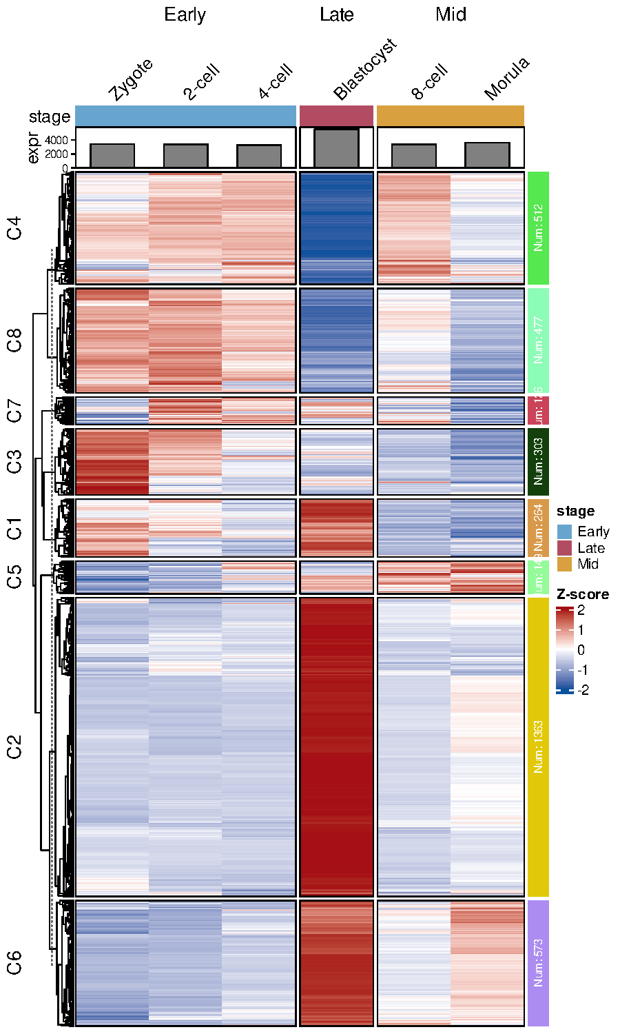
# 3. heatmapAnnotation + columnSplit:多重列注释 + 列拆分
#    ⚠ 一旦传 heatmapAnnotation, 列注释完全交给用户
#      (sampleGroup/sampleCol 失效);columnSplit 按组拆列(组间留白)
# ------------------------------------------------------------
ha <- ComplexHeatmap::HeatmapAnnotation(
  stage = c("Early", "Early", "Early", "Mid", "Mid", "Late"),
  expr = ComplexHeatmap::anno_barplot(colSums(exps)),
  col = list(stage = c(Early = "#67A5CE", Mid = "#D8A03E", Late = "#B24C63")),
  annotation_name_side = "left")
p_ha <- visCluster(ck, plotType = "heatmap",
                   column_names_rot = 45,
                   heatmapAnnotation = ha,
                   columnSplit = c("Early", "Early", "Early",
                                   "Mid", "Mid", "Late"))
save_ht_pdf(p_ha, "../output/28_heatmap_heatmapAnnotation.pdf",
            width = 6, height = 10)
cat("28 heatmapAnnotation+columnSplit OK\n")

# ------------------------------------------------------------
# 4. sampleOrder:列(时间点/样本)自定义排序(折线图与热图均生效)
#    例: 把 Blastocyst 挪到最前(演示用;实战用于统一多图列序)
# ------------------------------------------------------------
p_so <- visCluster(ck, plotType = "line",
                   sampleOrder = c("Blastocyst", "Zygote", "2-cell",
                                   "4-cell", "8-cell", "Morula"))
ggplot2::ggsave("../output/29_line_sampleOrder.pdf", p_so,
                width = 10, height = 6)
cat("29 sampleOrder 列排序 OK\n")

# ------------------------------------------------------------
# 5. rowAnnotationObj:自定义左侧行注释(rowAnnotation 对象)
#    例: 每个基因的平均表达 barplot(注意行序与 mat 一致: ck$wide.res 已按簇排好)
# ------------------------------------------------------------
mat_rows <- ck$wide.res$gene
foo_val <- rowMeans(as.matrix(ck$wide.res[, grepl("cell|Zygote|Morula|Blastocyst",
                                                  colnames(ck$wide.res))]))
ra <- ComplexHeatmap::rowAnnotation(
  avgExpr = ComplexHeatmap::anno_barplot(foo_val,
                                         gp = grid::gpar(fill = "#4DBBD5"),
                                         width = grid::unit(2, "cm")))
p_ra <- visCluster(ck, plotType = "heatmap",
                   column_names_rot = 45,
                   rowAnnotationObj = ra)   # 放到热图左侧
save_ht_pdf(p_ra, "../output/30_heatmap_rowAnnotationObj.pdf",
            width = 7, height = 10)
cat("30 rowAnnotationObj 左侧注释 OK\n")

# ------------------------------------------------------------
# 6. 其他微调开关
# ------------------------------------------------------------
# 6a. clusterColumns=TRUE: 列聚类(默认 FALSE, 保持时间序)
p_cc <- visCluster(ck, plotType = "heatmap",
                   column_names_rot = 45,
                   clusterColumns = TRUE)
save_ht_pdf(p_cc, "../output/31_heatmap_clusterColumns.pdf",
            width = 5, height = 10)
cat("31 clusterColumns OK\n")

# 6b. addSampleAnno=FALSE: 去掉顶部样本色条; annnoblockText=FALSE: 去掉右侧 Num 数字
p_na <- visCluster(ck, plotType = "heatmap",
                   column_names_rot = 45,
                   addSampleAnno = FALSE,
                   annnoblockText = FALSE)
save_ht_pdf(p_na, "../output/32_heatmap_noAnno.pdf", width = 5, height = 10)
cat("32 addSampleAnno=F + annnoblockText=F OK\n")

# 6c. byGo="anno_block": GO 注释用块状文本框(而非 anno_link 连线式, 10.2 已演示)
data(termanno)
p_blk <- visCluster(ck, plotType = "both",
                    column_names_rot = 45,
                    annoTermData = termanno,
                    byGo = "anno_block")
save_ht_pdf(p_blk, "../output/33_both_GO_annoBlock.pdf", width = 9, height = 10)
cat("33 byGo=anno_block OK\n")

cat("10.6 全部完成\n")

#!/usr/bin/env Rscript
# ============================================================
# ClusterGVis 富集与数据准备补遗(10.2/10.3 未覆盖的参数分支):
#   1. enrichCluster type=MF / CC            GO 另两个本体
#   2. enrichCluster topn 向量               每簇不同条数
#   3. enrichCluster type=ownSet             自定义基因集(TERM2GENE)
#   4. enrichCluster 直入 CellDataSet        monocle2 cds 一站式
#   5. clusterData subcluster                只保留部分簇
#   6. clusterData kmeansParamsList/TCseqParamsList   算法参数透传
#   7. clusterData minStd / scaleData        过滤与不 z-score
#   8. prepareDataFromscRNA groupBy/keepUniqGene=FALSE/cells
# 输出:全部 PDF(矢量),写入 ../output/
# ============================================================
suppressPackageStartupMessages({
  library(ClusterGVis)
  library(ComplexHeatmap)
  library(org.Mm.eg.db)   # exps 是小鼠胚胎数据
  library(dplyr)
})

dir.create("../output", showWarnings = FALSE)
save_ht_pdf <- function(ht, file, width = 6, height = 10) {
  grDevices::cairo_pdf(file, width = width, height = height, onefile = FALSE)
  ComplexHeatmap::draw(ht)
  grDevices::dev.off()
}

data(exps)
ck <- clusterData(obj = exps, clusterMethod = "kmeans", clusterNum = 8)

# ------------------------------------------------------------
# 1. enrichCluster type=MF / CC(10.2 只演示了 BP;用法完全一致)
# ------------------------------------------------------------
en_mf <- enrichCluster(ck, OrgDb = org.Mm.eg.db, type = "MF",
                       pvalueCutoff = 0.05, topn = 2)
en_cc <- enrichCluster(ck, OrgDb = org.Mm.eg.db, type = "CC",
                       pvalueCutoff = 0.05, topn = 2)
cat("1. MF:", nrow(en_mf), "行 / CC:", nrow(en_cc), "行\n")
write.csv(en_mf, "../output/enrichCluster_MF_top2.csv", row.names = FALSE)
write.csv(en_cc, "../output/enrichCluster_CC_top2.csv", row.names = FALSE)

# ------------------------------------------------------------
# 2. topn 向量:每簇取不同条数(长度须 = 簇数)
# ------------------------------------------------------------
en_vec <- enrichCluster(ck, OrgDb = org.Mm.eg.db, type = "BP",
                        pvalueCutoff = 0.05,
                        topn = c(3, 2, 4, 2, 3, 2, 5, 2))   # C1..C8 各取 n 条
cat("2. topn 向量 每簇条数:", paste(table(en_vec$group), collapse = "/"), "\n")

# ------------------------------------------------------------
# 3. type="ownSet":自定义基因集富集(无需 OrgDb, 离线可用)
#    TERM2GENE: 两列 term/gene;TERM2NAME 可选(term -> 展示名)
#    实战: 传入 MSigDB/自研 signature;演示用随机分组模拟
#    ⚠ idTrans 必须设 FALSE(基因名已是 SYMBOL, 不做 ID 转换)
# ------------------------------------------------------------
set.seed(1)
genes.all <- rownames(exps)
t2g <- data.frame(
  term = rep(c("CellCycle", "Metabolism", "Signaling", "ECM", "Stemness"),
             each = 120),
  gene = sample(genes.all, 600))
t2n <- data.frame(
  term = c("CellCycle", "Metabolism", "Signaling", "ECM", "Stemness"),
  name = c("细胞周期", "代谢", "信号转导", "细胞外基质", "干性"))
ck3 <- clusterData(exps, clusterMethod = "kmeans", clusterNum = 3)
en_own <- enrichCluster(ck3, type = "ownSet",
                        TERM2GENE = t2g, TERM2NAME = t2n,
                        idTrans = FALSE,
                        pvalueCutoff = 1,   # 演示基因集小, 放宽阈值
                        topn = 2)
cat("3. ownSet:", nrow(en_own), "行\n")
print(head(en_own, 3))
write.csv(en_own, "../output/enrichCluster_ownSet_top2.csv", row.names = FALSE)

# ------------------------------------------------------------
# 4. enrichCluster 直入 CellDataSet(monocle2 一站式: 拟时序热图聚类 -> 富集)
#    ⚠ 包 bug 提示: heatmapType 选 "plot_multiple_branches_heatmap2"
#      实际会 fallback 调 plot_pseudotime_heatmap2(源码写死), 该函数并不存在
#    ⚠ HSMM(人源)用 org.Hs.eg.db + fromType="SYMBOL";富集内部对 cds
#      先跑拟时序热图聚类再逐簇 bitr, 耗时较长属正常
# ------------------------------------------------------------
suppressPackageStartupMessages({library(monocle); library(org.Hs.eg.db)})
data(HSMM)
en_cds <- enrichCluster(HSMM, type = "BP", OrgDb = org.Hs.eg.db,
                        fromType = "SYMBOL",
                        heatmapType = "plot_pseudotime_heatmap2",
                        num_clusters = 3, norm_method = "vstExprs")
cat("4. cds 直入富集:", nrow(en_cds), "行\n")
print(head(en_cds[, c("group", "Description", "pvalue")], 3))
write.csv(en_cds, "../output/enrichCluster_cds_BP.csv", row.names = FALSE)

# ------------------------------------------------------------
# 5. subcluster:聚类时只保留指定簇(如只关心下调模块 C1/C3)
# ------------------------------------------------------------
ck_sub <- clusterData(exps, clusterMethod = "kmeans",
                      clusterNum = 8, subcluster = c(1, 3))
cat("5. subcluster 保留簇:", paste(unique(ck_sub$wide.res$cluster), collapse = ","),
    "(共", nrow(ck_sub$wide.res), "基因)\n")
p_sub <- visCluster(ck_sub, plotType = "both", column_names_rot = 45)
save_ht_pdf(p_sub, "../output/34_both_subcluster.pdf", width = 7, height = 8)
cat("34 subcluster 出图 OK\n")

# ------------------------------------------------------------
# 6. kmeansParamsList / TCseqParamsList:算法参数透传
#    kmeans -> stats::kmeans(nstart/iter.max/...);TCseq -> timeclust(...)
#    nstart 越大结果越稳定(多初始中心取最优)
# ------------------------------------------------------------
ck_p50 <- clusterData(exps, clusterMethod = "kmeans", clusterNum = 8,
                      kmeansParamsList = list(nstart = 50, iter.max = 100))
cat("6. kmeansParamsList(nstart=50) 簇大小:",
    paste(table(ck_p50$wide.res$cluster), collapse = "/"), "\n")

ct_p <- clusterData(exps, clusterMethod = "TCseq", clusterNum = 8,
                    TCseqParamsList = list(iter.max = 50))
cat("   TCseqParamsList(iter.max=50) 簇数:",
    length(unique(ct_p$wide.res$cluster)), "\n")

# ------------------------------------------------------------
# 7. minStd / scaleData:低波动基因过滤 与 关闭 z-score
#    minStd: sd <= minStd 的基因先被 filter.std 剔除(mfuzz/TCseq/kmeans 均走此步)
#    scaleData=FALSE: 不做 z-score, 热图展示原始表达(TPM/logCPM)
# ------------------------------------------------------------
cm_f <- clusterData(exps, clusterMethod = "mfuzz", clusterNum = 8, minStd = 0.5)
cat("7. mfuzz minStd=0.5 过滤后:", nrow(cm_f$wide.res), "基因(原 3767)\n")

ck_ns <- clusterData(exps, clusterMethod = "kmeans", clusterNum = 8,
                     scaleData = FALSE)
p_ns <- visCluster(ck_ns, plotType = "heatmap", column_names_rot = 45,
                   htColList = list(col_range = c(0, 500, 1000),   # 原始尺度自行调范围
                                    col_color = c("#08519C", "white", "#A50F15")))
save_ht_pdf(p_ns, "../output/35_heatmap_noScale.pdf", width = 5, height = 10)
cat("35 scaleData=FALSE OK\n")

# ------------------------------------------------------------
# 8. prepareDataFromscRNA 其余参数
#    groupBy: 按任意 meta 列分组(默认 ident)
#    keepUniqGene=FALSE: 跨簇重复基因保留(名字加后缀, geneType="nounique")
#    cells: 只取指定细胞子集
# ------------------------------------------------------------
suppressPackageStartupMessages(library(Seurat))
data(pbmc_subset)
Idents(pbmc_subset) <- "seurat_clusters"
mk.all <- FindAllMarkers(pbmc_subset, only.pos = TRUE,
                         min.pct = 0.25, logfc.threshold = 0.25)
mk <- mk.all |> group_by(cluster) |> top_n(n = 10, wt = avg_log2FC)

# 8a. keepUniqGene=FALSE: 重复基因保留 -> wide.res 行数 > unique 基因数
st_nu <- prepareDataFromscRNA(pbmc_subset, diffData = mk,
                              showAverage = TRUE, keepUniqGene = FALSE)
cat("8a. keepUniqGene=FALSE geneType:", st_nu$geneType,
    " 行数:", nrow(st_nu$wide.res), "\n")

# 8b. groupBy="seurat_clusters"(等价默认 ident, 演示任意列)
st_grp <- prepareDataFromscRNA(pbmc_subset, diffData = mk,
                               showAverage = TRUE, groupBy = "seurat_clusters")
cat("8b. groupBy 列分组 OK, 列名:", paste(colnames(st_grp$wide.res)[1:3],
                                          collapse = ","), "...\n")

# 8c. cells: 只取前 500 个细胞(单细胞级热图场景)
st_cells <- prepareDataFromscRNA(pbmc_subset,
                                 diffData = mk[, c("cluster", "gene")],
                                 showAverage = FALSE,
                                 cells = head(colnames(pbmc_subset), 500))
cat("8c. cells 子集列数:", ncol(st_cells$wide.res) - 2, "\n")

cat("10.7 全部完成\n")